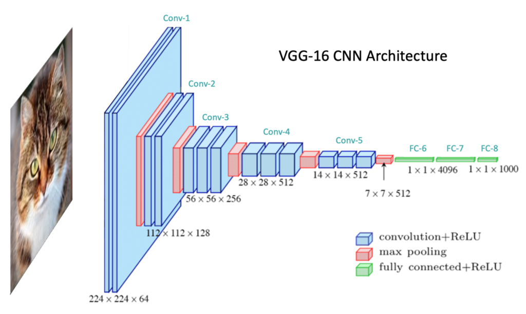
Convolutional Neural Network (CNN): A Complete Guide

Convolutional Neural Network (CNN) forms the basis of computer vision and image processing. In this post, we will learn about Convolutional Neural Networks in the context of an image classification problem. We first cover the basic structure of CNNs and then go into the detailed operations of the various layer types commonly used. The above diagram shows the network architecture of a well-known CNN called VGG-16 for illustration purposes. It also shows the general structure of a CNN, which typically includes a series of convolutional blocks followed by a number of fully connected layers.

The convolutional blocks extract meaningful features from the input image, passing through the fully connected layers for the classification task.

• Motivation
• Convolutional Neural Network (CNN) Architecture Components
• Convolutional Blocks and Pooling Layers
• Fully Connected Classifier
• Conclusion

Motivation

In an earlier post on image classification, we used a densely connected Multilayer Perceptron (MLP) network to classify handwritten digits. However, one problem with using a fully connected MLP network for processing images is that image data is generally quite large, which leads to a substantial increase in the number of trainable parameters. This can make it difficult to train such networks for a number of reasons.

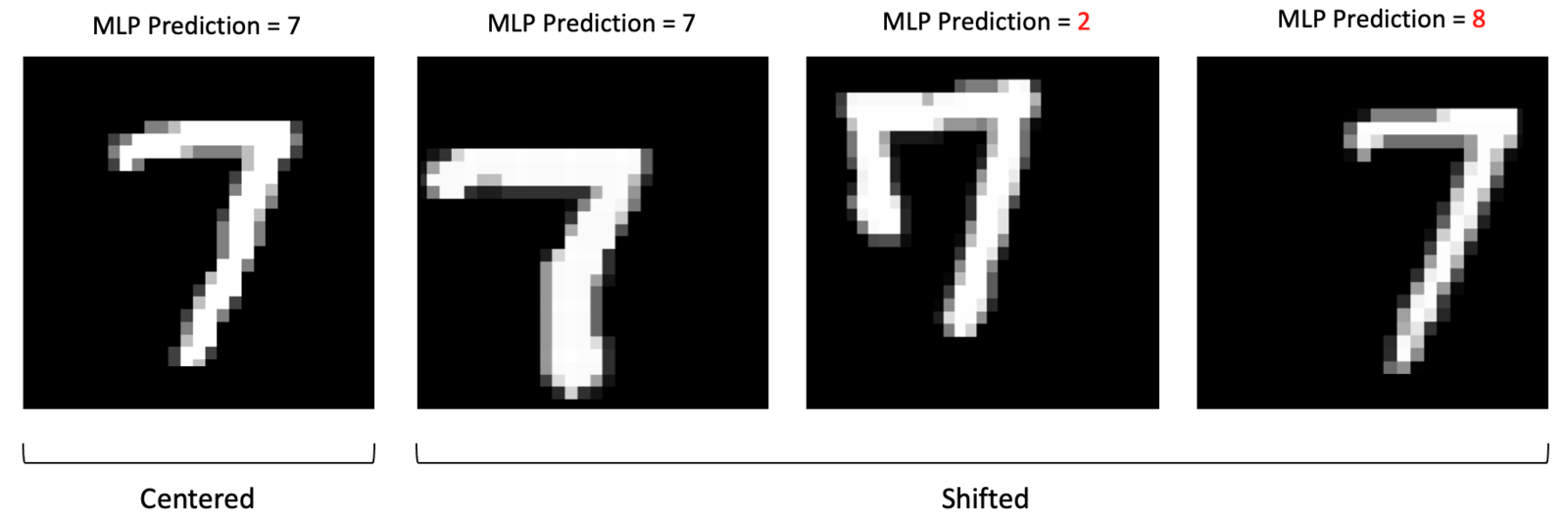
MLPs are Not Translation Invariant

One issue with using MLPs to process image data is that they are not translation invariant. This means that the network reacts differently if the main content of the image is shifted. Since MLPs respond differently to shifted images, the examples below illustrate how such images complicate the classification problem and produce unreliable results.

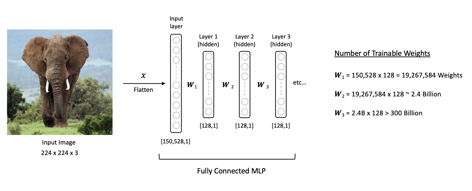
MLPs are Prone to Overfitting

Another issue with processing image data with MLPs is that MLPs use a single neuron for every input pixel in the image. So the number of weights in the network rapidly becomes unmanageable (especially for large images with multiple channels). Take, for example, a color image with a size of (224x244x3). The input layer in an MLP would have 150,528 neurons. If we then have just three modest size hidden layers with 128 neurons each followed by the input layer, we would exceed 300 Billion trainable parameters in the network! Not only would the training time be exceedingly large for such a network, but the model would also be highly prone to overfitting the training data due to such a large number of trainable parameters.

Convolutional Neural Network (CNN)

Fortunately, there are better ways to process image data. Convolutional Neural Networks (CNN) were developed to more effectively and efficiently process image data. This is largely due to the use of convolution operations to extract features from images. This is a key feature of convolutional layers, called parameter sharing, where the same weights are used to process different parts of the input image. This allows us to detect feature patterns that are translation invariant as the kernel moves across the image. This approach improves the model efficiency by significantly reducing the total number of trainable parameters compared to fully connected layers.

Let’s now look at VGG-16 to study the architectural components and the operations associated with individual layers.

Convolutional Neural Network (CNN) Architecture Components

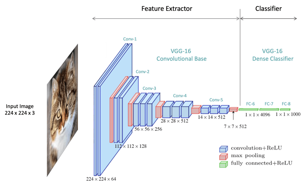
VGG-16 CNN Architecture

At a high level, CNN architectures contain an upstream feature extractor followed by a downstream classifier. The feature extraction segment is sometimes referred to as the “backbone” or “body” of the network. The classifier is sometimes referred to as the “head” of the network.

In this section, we will introduce all the layer types that form the basis of both network components. To facilitate the discussion, we will refer to VGG-16 CNN architecture, as shown in the figure below.

The model begins with five convolutional blocks, constituting the model’s feature extraction segment. A convolutional block is a general term used to describe a sequence of layers in a CNN that are often repeatedly used in the feature extractor. The feature extractor is followed by the classifier, which transforms the extracted features into class predictions in the final output layer. VGG-16 was trained on the ImageNet dataset, which contains 1,000 classes. Therefore, the output layer contains 1,000 neurons whose values represent the probabilities that the input image corresponds to each class. The output with the highest probability is, therefore, the predicted class.

Notice that the layers depicted in the architecture each have a spatial dimension and a depth dimension. These dimensions represent the shape of the data as it flows through the network. The VGG-16 network is specifically designed to accept color images with an input shape of 224x224x3, where the 3 represents the RGB color channels. As the input data passes through the network, the shape of the data is transformed. The spatial dimensions are (intentionally reduced) while the depth of the data is increased. The depth of data is referred to as the number of channels.

 Convolutional Blocks and Pooling Layers

The figure below is another way to depict the layers in a network visually. In the case of VGG-16, there are five convolutional blocks (Conv-1 to Conv-5). The specific layers within a convolutional block can vary depending on the architecture. However, a convolutional block typically contains one or more 2D convolutional layers followed by a pooling layer. Other layers are also sometimes incorporated, but we will focus on these two layer types to keep things simple.

Notice that we have explicitly specified the last layer of the network as SoftMax. This layer applies the softmax function to the outputs from the last fully connected layer in the network (FC-8). It converts the raw output values from the network to normalized values in the range [0,1], which we can interpret as a probability score for each class.

Convolutional Layers

A convolutional layer can be thought of as the “eyes” of a CNN. The neurons in a convolutional layer look for specific features. At the most basic level, the input to a convolutional layer is a two-dimensional array which can be the input image to the network or the output from a previous layer in the network. The input to the very first convolutional layer is the input image. The input image is typically either a grayscale image (single channel) or a color image (3 channels).

In the case of VGG-16, the input is a color image with the shape: (224x224x3). Here we depict a high-level view of a convolutional layer. Convolutional layers use filters to process the input data. The filter moves across the input, and at each filter location, a convolution operation is performed, which produces a single number. This value is then passed through an activation function, and the output from the activation function populates the corresponding entry in the output, also known as an activation map (224x224x1). You can think of the activation map as containing a summary of features from the input via the convolution process.

The Convolution Operation (Input * Kernel)

Before we can describe convolutional layers in more detail, we need first to take a small detour to explain how the convolution operation is performed. In a convolutional layer, a small filter is used to process the input data. In this example, we show how (6x6) input is convolved with a (3x3) filter. Here we show a simple filter often used in image processing. The elements in a filter are collectively referred to as a kernel. Here we will use a well-known kernel often used in image processing called a Sobel kernel which is designed to detect vertical edges. However, it’s important to note that in CNNs, the elements in the kernel are weights that are learned by the network during training.

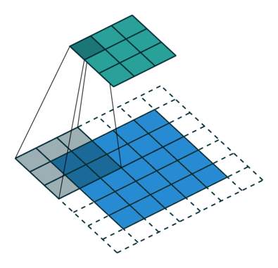
The convolution operation consists of placing the kernel over a portion of the input and multiplying the elements of the filter with the corresponding elements of the input. The resulting value is a single number representing the output of the convolution operation for a given filter location. The process is repeated by sliding the filter over the input image until the filter has been placed over each input section. Sliding the filter one pixel at a time corresponds to a stride of one. The filter location is shown in dark blue. This region is also referred to as the receptive field. Notice that the center of the filter is indicated in green. The convolution operation performed at each filter location is simply the dot product of the filter values with the corresponding values in the receptive field in the input data.

A sample calculation is provided for the first two filter locations so you can confirm your understanding of the operation. Notice that at each filter location, the operation produces a single number placed at the corresponding location in the output (i.e., the location in the output that corresponds to the center of the receptive field overlayed on the input slice).

Stride

Stride determines how many pixels the kernel shifts over the input at a time. For example, a stride of 1 means the dot product is performed on an n x n window of the 2D input, then shifts kernel by one pixel for subsequent operation across both axes. Decreasing the stride length results in learning more features and larger output layers due to more feature extraction. On the contrary, increasing the stride results in reduced output layer dimensions. 

Padding

Padding is an important parameter in CNN, which helps to preserve the input spatial dimension by adding extra pixels around the input image borders. By conserving border information, helps to improve model performance in determining the output spatial size of feature maps.

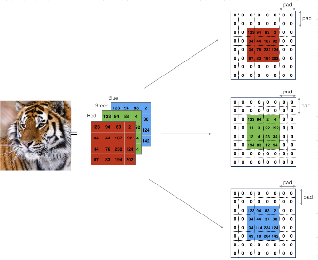
There are several padding techniques like zero padding, same padding, valid padding etc., but zero padding is widely used because it is simple and computationally efficient. It involves adding zeros symmetrically around edges of the input matrix as in high performance architectures like AlexNet.

Convolution Output Spatial Size

A 2D Convolution output feature size is determined by the formula,

where, 

• O: Output size
• n: Input size (height or width)
• f:  kernel size
• p: Padding
• s: Stride

Suppose you have a 32×32 input with 3×3 kernel (f), same padding (p = 1 ) and No stride (i.e. s = 1)

The output feature map size is calculated as follows:

Therefore, the input spatial dimension is preserved without reducing the output layer dimension.

💡 To Do for Learner: Calculate the output feature size of a 64×64 input image with f = 3, valid padding (p=0), s = 1.

Sobel Kernel Example

Here we show a concrete example of how a Sobel Kernel detects vertical edges. Recall the convolution operation defined above is the weighted sum of the kernel values with the corresponding input values. Since the Sobel kernel has positive values in the left column, zeros in the center column, and negative values in the right column, as the kernel is moved from left to right across the image, the convolution operation is a numerical approximation of the derivative in the horizontal direction, and therefore, the output produced detects vertical edges. This is an example of how specific kernels can detect various structures in images like edges. Other kernels can be used to detect horizontal lines/edges or diagonal lines/edges. In CNN, this concept is generalized. Since the kernel weights are learned during the training process, CNNs can therefore learn to detect many types of features that support image classification.

Convolutional Layer Properties

Recall the output of the convolution operation is passed through an activation function to produce what are known as activation maps. Convolutional layers typically contain many filters, meaning each convolutional layer produces multiple activation maps. As image data is passed through a convolutional block, the net effect is to transform and reshape the data. Before we proceed, it’s worth noting the following points.

• The depth of a filter (channels) must match the depth of the input data (i.e., the number of channels in the input).
• The spatial size of the filter is a design choice but 3x3 is very common (or sometimes 5x5).
• The number of filters is also a design choice and dictates the number of activation maps produced in the output.
• Multiple activations maps are sometimes collectively referred to as “an activation map containing multiple channels.” But we often refer to each channel as an activation map.
• Each channel in a filter is referred to as a kernel so that you can think of a filter as a container for kernels.
• A single-channel filter has just one kernel. Therefore, in this case, the filter and the kernel are one and the same.
• The weights in a filter/kernel are initialized to small random values and are learned by the network during training.
• The number of trainable parameters in a convolutional layer depends on the number of filters, the filter size, and the number of channels in the input.

Convolutional Layer with a Single Filter

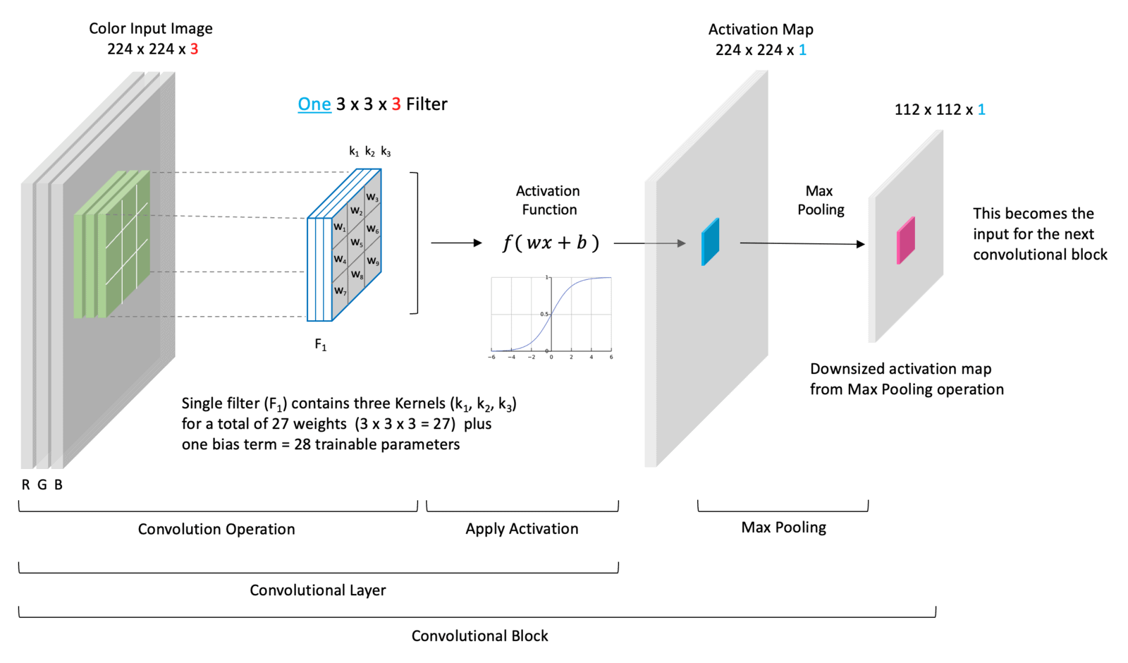
Let’s now look at a concrete example of a simple convolutional layer. Suppose the input image has a size of (224x224x3). The spatial size of a filter is a design choice, but it must have a depth of three to match the depth of the input image. In this example, we use a single filter of size (3x3x3).

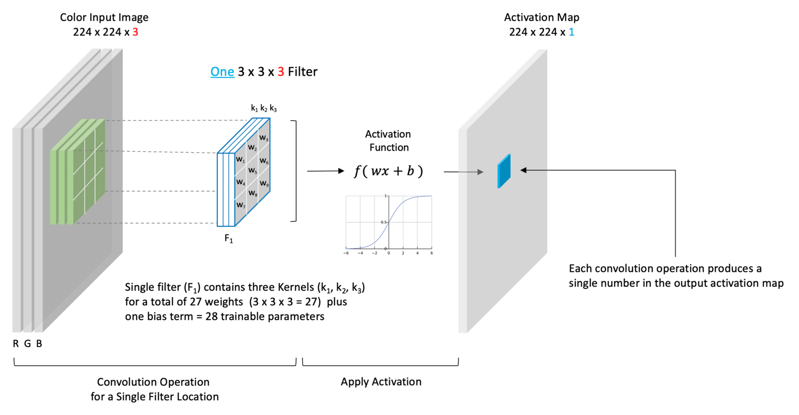
Here we have chosen to use just a single filter. Therefore the filter contains three kernels where each kernel has nine trainable weights. There are a total of 27 trainable weights in this filter, plus a single bias term, for 28 total trainable parameters. Because we’ve chosen just a single filter, the depth of our output is one, which means we produce just a single channel activation map shown. When we convolve this single (3-channel) filter with the (3-channel) input, the convolution operation is performed for each channel separately. The weighted sum of all three channels plus a bias term is then passed through an activation function whose output is represented as a single number in the output activation map (shown in blue).

So to summarize, the number of channels in a filter must match the number of channels in the input. The number of filters in a convolutional layer (a design choice) dictates the number of activation maps that are produced by the convolutional layer.

In practice, convolutional layers often contain many filters. To reinforce the implications of this, consider a convolutional layer with 32 filters. Such a layer will produce 32 activation maps. An adjacent (subsequent) convolutional layer could contain any number of filters (a design choice). However, the number of channels in those filters must be 32 to match the depth of the input (the output from the previous layer).

Convolutional Layer with Two Filters

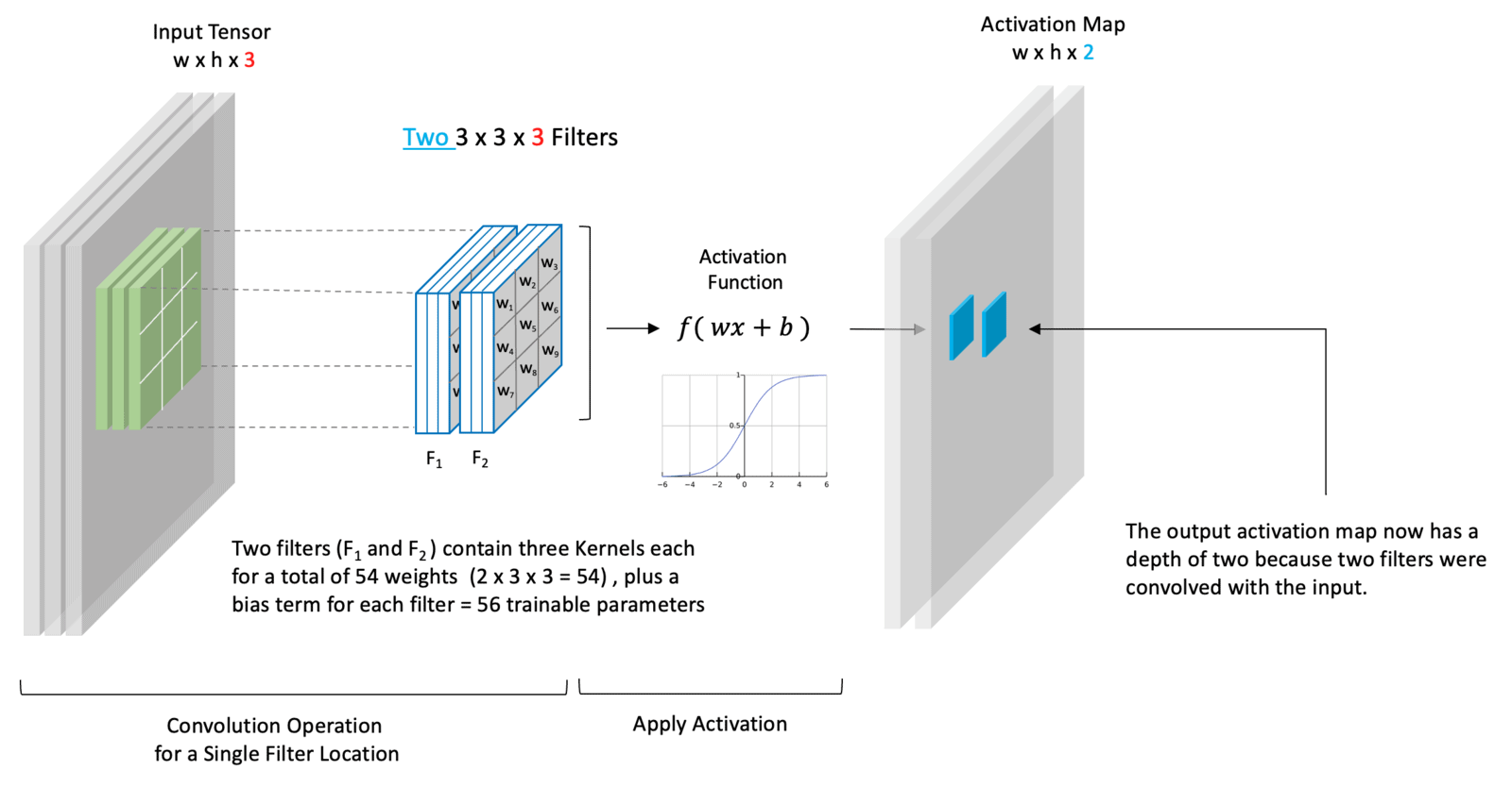
This next example represents a more general case. First, notice that the input has a depth of three, but this doesn’t necessarily correspond to color channels. It just means that we have an input tensor that has three channels. Remember that when we refer to the input, we don’t necessarily mean the input to the neural network but rather the input to this convolutional layer which could represent the output from a previous layer in the network.

In this case, we’ve chosen to use two filters. Because the input depth is three, each filter must have a depth of three. This means that there are 54 trainable weights because each filter contains 27 weights. We also have one bias term for each filter, so we have a total of 56 trainable parameters.

Filters Learn to Detect Structure

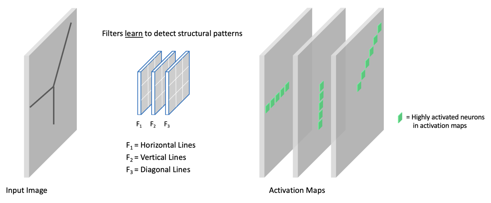
You can think of each filter in a convolutional layer as learning something special and unique about the input data. Remember that each filter contains weights that are learned during the training process. The individual channels in the activation maps at any point in the network represent features extracted from the input image. Here we show an input image with various linear (edge) components. In this example, we have a convolutional layer with three filters. Each filter learns to detect different structural elements (i.e., horizontal lines, vertical lines, and diagonal lines). To be more precise, these “lines” represent edge structures in an image. In the output activation maps, we emphasize the highly activated neurons associated with each filter.

CNNs Learn Hierarchical Features

In 2013, a seminal paper Visualizing and Understanding Convolutional Networks shed light on why CNNs perform so well. They introduced a novel visualization technique that gives insight into the function of intermediate layers within a CNN model.

In the diagram below, we take two examples from the paper to illustrate that the filters in the first layer learn to detect basic structural elements like edges and color blobs, while layers deeper in the network are able to detect more complex compositional structures.

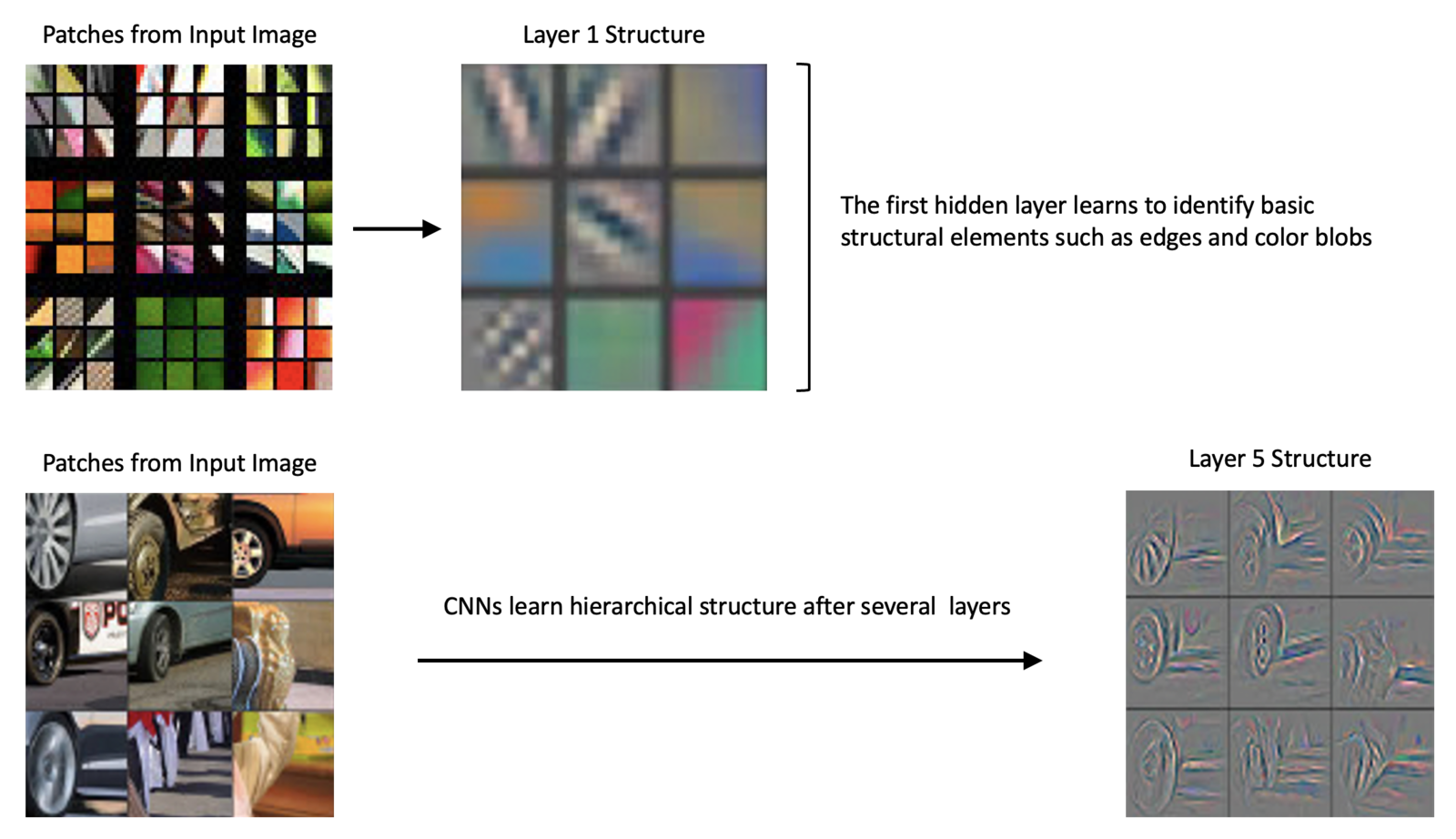
The following notes are from the original paper:

Visualization of features in a fully trained model. The top 9 activations in a random subset of feature maps across the validation data, projected down to pixel space using our deconvolutional network approach. Our reconstructions are not samples from the model: they are reconstructed patterns from the validation set that cause high activations in a given feature map. For each feature map, we also show the corresponding image patches.

Max Pooling Layers

In CNN architectures, it is typical that the spatial dimension of the data is reduced periodically via pooling layers. Pooling layers are typically used after a series of convolutional layers to reduce the spatial size of the activation maps. You can think of this as a way to summarize the features from an activation map. Using a pooling layer will reduce the number of parameters in the network because the input size to subsequent layers is reduced. This is a desirable effect because the computations required for training are also reduced. Also, using fewer parameters often helps to mitigate the effects of overfitting.

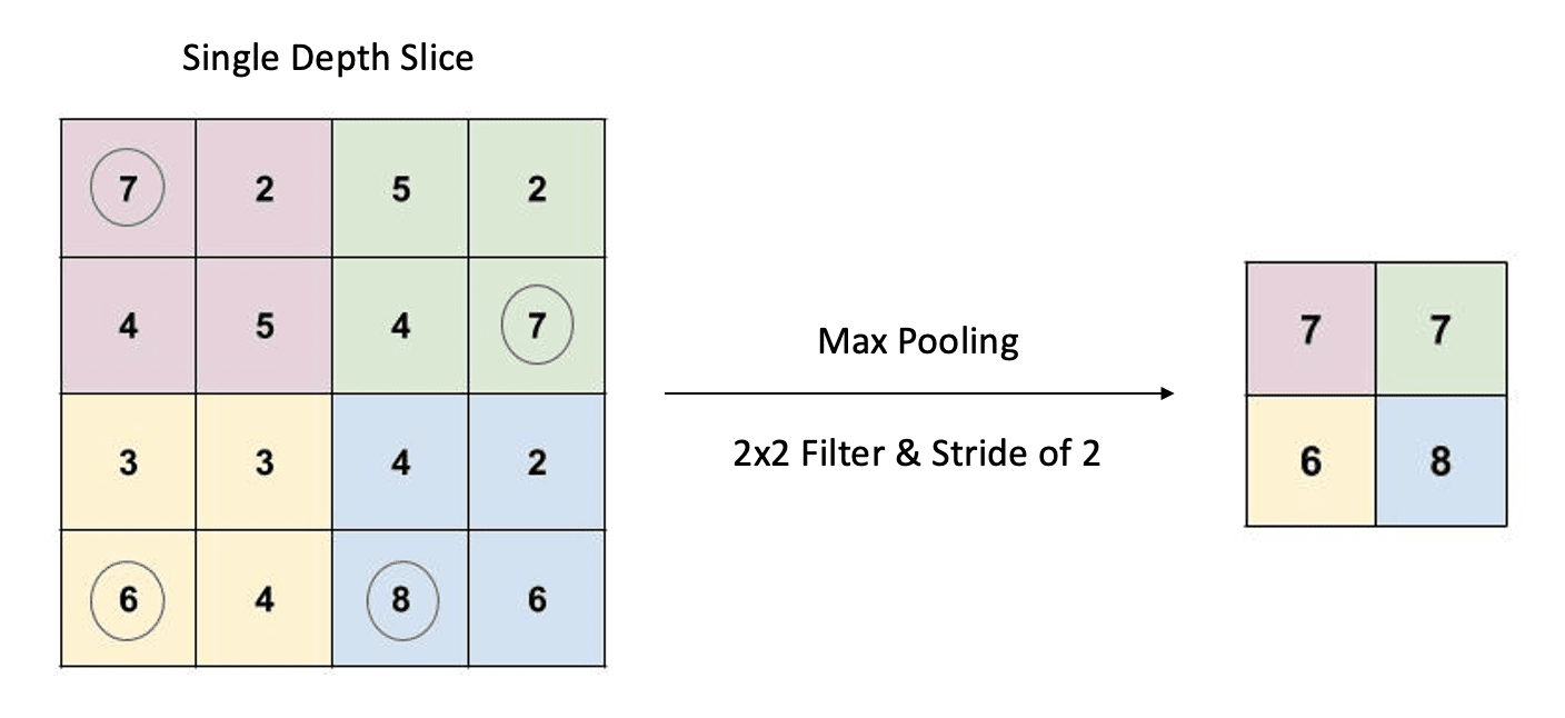
Pooling is a form of downsizing that uses a 2D sliding filter. The filter passes over the input slice according to a configurable parameter called the stride. The stride is the number of pixels the filter moves across the input slice from one position to the next. The are two types of pooling operations: average pooling and max pooling. However, max pooling is the most common.

For any given filter location, the corresponding values in the input slice are passed through a max() operation. The maximum value is then recorded in the output. As shown in the example above, we have a 4x4 input slice, a 2x2 filter, and a stride of two. The corresponding output is, therefore, a 2x2 down-sized representation of the input slice.

Contrary to convolutional filters, the filter in a pooling layer has no trainable parameters. The filter specifies the size of the window used to perform the max() operation.

Convolutional Block Detail (Example)

Let’s now look at what a very simple convolutional block looks like at the beginning of a network. For simplicity, we show a single convolutional layer containing a single filter. The input to the layer is the input image. In the case of VGG-16, this is a color image indicated by the three RGB channels. After the convolutional layer, a max pooling layer is added to reduce the spatial dimension of the activation map.

The only difference between this diagram and the convolutional blocks used in CNN architectures like VGG-16 is that there are usually two or three consecutive convolutional layers followed by a max pooling layer. And convolutional layers usually contain at least 32 filters.

Neuron Connectivity in CNNs

Due to the complexity of CNNs, most diagrams do not depict individual neurons and their weighted connections. It’s difficult to depict this visually since the weights in the filters are shared by multiple neurons in the input to a convolutional layer. However, notice that each neuron in the output activation map is only connected to nine neurons in the input volume via the filter’s nine weights. In other words, each neuron in the output layer only looks at a small portion of the input image defined by the spatial size of the filter. This region in the input image is known as the receptive field (shown in Green). The receptive field defines the spatial extent of the connectivity between the output and input for a given filter location. 

To summarize, the input neurons to a convolutional layer are connected to the neurons in the activation map(s) via the shared weights in the filter(s).

Fully Connected Classifier

The fully connected (dense) layers in a CNN architecture transform features into class probabilities. In the case of VGG-16, the output from the last convolutional block (Conv-5) is a series of activation maps with shape (7x7x512). For reference, we have indicated the number of channels at key points in the architecture.

Before the data from the last convolutional layer in the feature extractor can flow through the classifier, it needs to be flattened to a 1-dimensional vector of length 25,088. After flattening, this 1-dimensional layer is then fully connected to FC-6, as shown below.

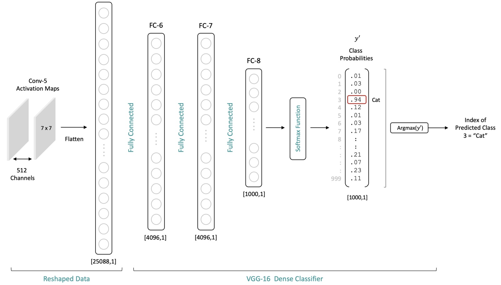
Let’s try to give some intuition for why the fully connected layers are needed and well-suited for the classification task. Remember that number of neurons in the output layer of the network is equal to the number of classes. Each output neuron is associated with a specific class. Each neuron’s value (after the softmax layer) represents the probability that the associated class for that neuron corresponds to the class associated with the input image.

Intuition for Why CNNs Work

The activation maps from the final convolutional layer of a trained CNN network represent meaningful information regarding the content of a particular image. Remember that each spatial location in a feature map has a spatial relationship with the original input image. Therefore, using fully connected layers in the classifier allows the classifier to process content from the entire image. Connecting the flattened output from the last convolutional layer in a fully connected manner to the classifier allows the classifier to consider information from the entire image.

Note: Flattening the output of Conv-5 is required for processing the activation maps through the classifier, but it does not alter the original spatial interpretation of the data. It’s just a repacking of the data for processing purposes.

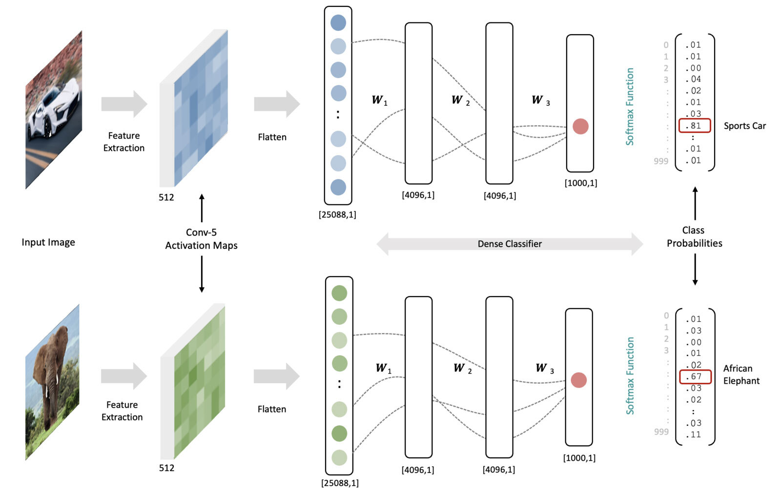
To make this more concrete, let’s assume we have a trained model (all the weights in the network are fixed). Now consider an input image of a car and an elephant. As the data for each image are processed through the network, the resulting feature maps at the last convolutional layer will look much different due to the input image content differences. When the final feature activation maps are processed through the classifier, combining the feature maps and the trained weights will lead to higher activations for the specific output neurons associated with each input image type. The (notional) dotted lines between the fully connected layers represent pathways leading to the highest activations in the output neurons (i.e., large weights coupled with high activations at each layer). In reality, there are over 100 Million connections between the flattened activation maps and the first fully connected layer in the classifier. And it’s worth emphasizing that the weights in both examples below are the same (they represent a trained network). The data in the figure below is notional to illustrate the concepts.

For anything larger than a toy problem, we can’t possibly internalize the thousands of mathematical operations that lead to this successful mapping, but at a high level, we understand that the weights in the network were trained in a principled way by minimizing a loss function, to learn meaningful features AND to “fire” the appropriate neuron in the output later. This is the essence of how such a network maps features to class probabilities.

Additional Topics in CNNs

Dropout

Dropout is a regularization technique that is applied to the fully connected layers or convolutional layers in CNNs to prevent overfitting by randomly setting a fraction of activations to zero during training; this encourages the network to develop more robust features without relying too much on weights of specific neurons. To learn more, read the next chapter of the guide, which explores this in detail.

Batch Normalization

Batch Normalization is another regularization technique used in CNNs to normalize the output of a previous activation layer by subtracting the batch mean and dividing by the batch standard deviation, followed by scaling and shifting. This process helps to stabilize and accelerate training by reducing internal covariate shifts and introduces slight noise in the network for better generalization. 

3D Convolution

For 3D convolution, the kernel shifts across three axes (height, width, and depth), allowing the capture of volumetric features in data such as medical imaging or video.

Summary of Key Points

We covered a lot of material in this notebook, so let’s summarize the key points.

• CNNs designed for a classification task contain an upstream feature extractor and a downstream classifier.
• The feature extractor comprises convolutional blocks with a similar structure composed of one or more convolutional layers followed by a max pooling layer.
• The convolutional layers extract features from the previous layer and store the results in activation maps.
• The number of filters in a convolutional layer is a design choice in the architecture of a model, but the number of kernels within a filter is dictated by the depth of the input tensor.
• The depth of the output from a convolutional layer (the number of activation maps) is dictated by the number of filters in the layer.
• Pooling layers are often used at the end of a convolutional block to downsize the activation maps. This reduces the total number of trainable parameters in the network and, therefore, the training time required. Additionally, this also helps mitigate overfitting.
• The classifier portion of the network transforms the extracted features into class probabilities using one or more densely connected layers.
• When the number of classes is more than two, a SoftMax layer is used to normalize the raw output from the classifier to the range [0,1]. These normalized values can be interpreted as the probability that the input image corresponds to the class label for each output neuron.

References

1. CS231n Convolutional Neural Networks for Visual Recognition
2. 📸 CNN Visualizer