


In this article, we will learn about feedforward Neural Networks, also known as Deep feedforward Networks or Multi-layer Perceptrons. They form the basis of many important Neural Networks being used in the recent times, such as Convolutional Neural Networks ( used extensively in computer vision applications ), Recurrent Neural Networks ( widely used in Natural language understanding and sequence learning) and so on. We will try to understand the important concepts involved in an intuitive and interactive way, without going into the mathematics involved. If you are interested in diving into deep learning but don’t have much background in statistics and machine learning, then this article is a perfect starting point.
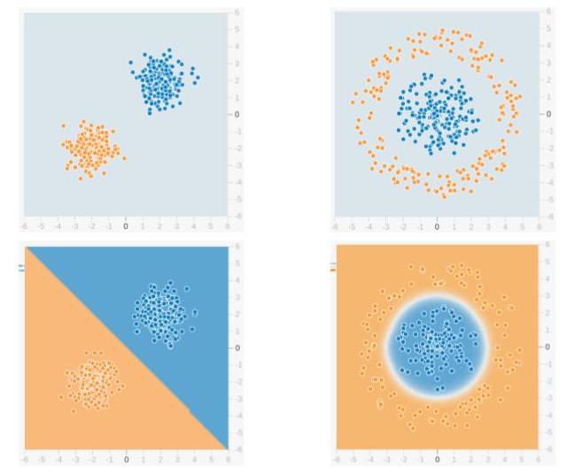
We will use the feedforward network to solve a binary classification problem. In Machine Learning, Classification is a type of Supervised Learning method, where the task is to divide the data samples into predefined groups by a Decision Function. When there are only two groups, it is called Binary Classification. The figure given below shows an example. The points in blue belong to one group ( or class ) and orange points belong to the other. The imaginary line(s) which separate the groups are called Decision Boundaries. The decision function is learned from a set of labeled samples, which is called Training Data and the process of learning the decision function is called Training.
In the above example, the top row shows two different data distributions and the bottom row shows the decision boundary. The left image shows an example of data which is Linearly Separable. This means that a linear boundary ( e.g. a straight line ) is enough to separate the data into groups. On the other hand, the image on the right shows an example of data which is not linearly separable. The decision boundary, in this case, has to be circular or polygonal as shown in the figure.
1. Understanding the Neural Network Jargon

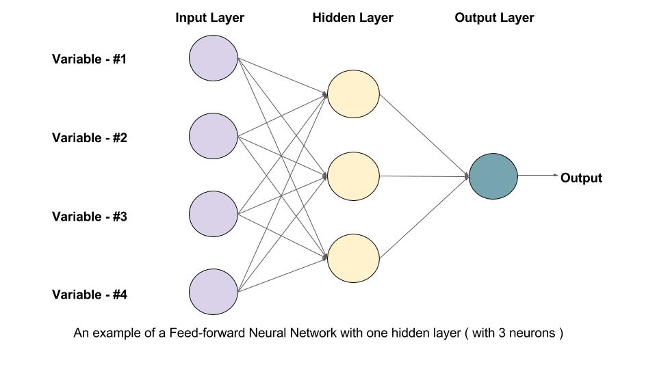
Given below is an example of a feedforward Neural Network. It is a directed acyclic Graph which means that there are no feedback connections or loops in the network. It has an input layer, an output layer, and a hidden layer. In general, there can be multiple hidden layers. Each node in the layer is a Neuron, which can be thought of as the basic processing unit of a Neural Network.


1.1. What is a Neuron?

An Artifical Neuron is the basic unit of a neural network. A schematic diagram of a neuron is given below.
As seen above, It works in two steps – It calculates the weighted sum of its inputs and then applies an activation function to normalize the sum. The activation functions can be linear or nonlinear. Also, there are weights associated with each input of a neuron. These are the parameters which the network has to learn during the training phase.
1.2. Activation Functions
The activation function is used as a decision making body at the output of a neuron. The neuron learns Linear or Non-linear decision boundaries based on the activation function. It also has a normalizing effect on the neuron output which prevents the output of neurons after several layers to become very large, due to the cascading effect. There are three most widely used activation functions
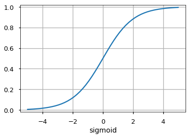
- Sigmoid
It maps the input ( x axis ) to values between 0 and 1.
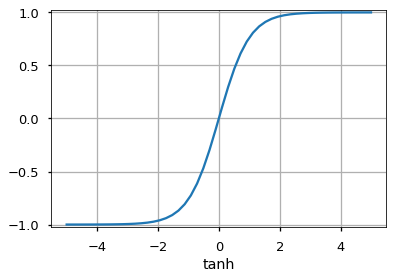
- Tanh
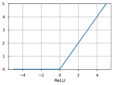
It is similar to the sigmoid function butmaps the input to values between -1 and 1. - Rectified Linear Unit (ReLU)
It allows only positive values to pass through it. The negative values are mapped to zero.
There are other functions like the Unit Step function, leaky ReLU, Noisy ReLU, Exponential LU etc which have their own merits and demerits.
1.3. Input Layer
This is the first layer of a neural network. It is used to provide the input data or features to the network.
1.4. Output Layer
This is the layer which gives out the predictions. The activation function to be used in this layer is different for different problems. For a binary classification problem, we want the output to be either 0 or 1. Thus, a sigmoid activation function is used. For a Multiclass classification problem, a Softmax ( think of it as a generalization of sigmoid to multiple classes ) is used. For a regression problem, where the output is not a predefined category, we can simply use a linear unit.
1.5. Hidden Layer
A feedforward network applies a series of functions to the input. By having multiple hidden layers, we can compute complex functions by cascading simpler functions. Suppose, we want to compute the 7th power of a number, but want to keep things simple ( as they are easy to understand and implement ). You can use simpler powers like square and cube to calculate the higher order functions. Similarly, you can compute highly complex functions by this cascading effect. The most widely used hidden unit is the one which uses a Rectified Linear Unit (ReLU) as the activation function.
The choice of hidden units is a very active research area in Machine Learning. The type of hidden layer distinguishes the different types of Neural Networks like CNNs, RNNs etc. The number of hidden layers is termed as the depth of the neural network. One question you might ask is exactly how many layers in a network make it deep? There is no right answer to this. In general, deeper networks can learn more complex functions.
1.6. How does the network learn?
The training samples are passed through the network and the output obtained from the network is compared with the actual output. This error is used to change the weights of the neurons such that the error decreases gradually. This is done using the Backpropagation algorithm, also called backprop. Iteratively passing batches of data through the network and updating the weights, so that the error is decreased, is known as Stochastic Gradient Descent ( SGD ). The amount by which the weights are changed is determined by a parameter called Learning rate. The details of SGD and backprop will be covered in a separate post.
2. Why use Hidden Layers?

To understand the significance of hidden layers we will try to solve the binary classification problem without hidden layers. For this, we will use an interactive platform from Google, playground.tensorflow.org which is a web app where you can create simple feedforward neural networks and see the effects of training in real time. You can play around by changing the number of hidden layers, number of units in a hidden layer, type of activation function, type of data, learning rate, regularization parameters etc. Given below is a screenshot of the web page.
In the above page, you can select the data and click on the play button to start training. It will show you the learned decision boundary and the loss curves at the top right corner.
2.1. No hidden layer
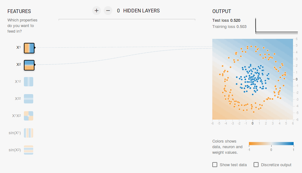
We want a network without a hidden layer which I have created in this link. Here there are no hidden layers so it becomes a simple neuron, which is capable of learning a linear decision boundary. We can select the type of data from the top left corner. In case of linearly separable data ( 3rd type ), it will be able to learn ( when you click the play button ) a linear boundary as shown below.

However, if you choose the 1st data it will not be able to learn the circular decision boundary.
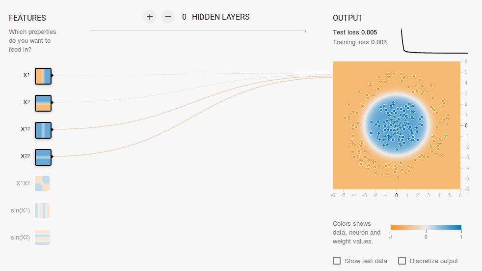
Since the data lies in a circular region, one may say that using squared values of the features as inputs might help. As it turns out, upon training, the neuron will be able to find the circular decision boundary.
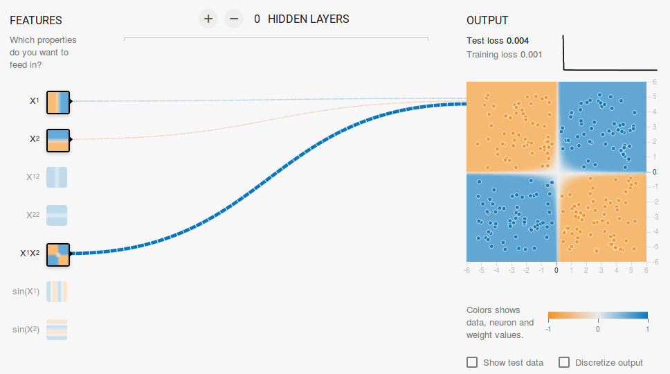
Now, if you select the 2nd data, the same configuration will not be able to learn the appropriate decision boundary.

Again by intuition, it looks like the decision boundary is a conic section( like a parabola or hyperbola ). So, if we include the product of the feature ( i.e. X1X2 ), the neuron is able to learn the desired decision boundary.
From the above experiment, we observed the following:
- Using a single neuron we can only learn a linear decision boundary
- We had to come up with feature transformations (like square of features or product of features) by visualizing the data. This step can be tricky for data which is not easy to visualize.
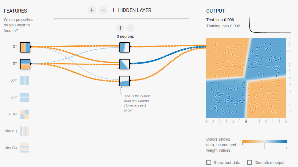
2.2. Adding a hidden layer
By adding a hidden layer as shown in this link, we can get rid of this feature engineering and have a single network which can learn all the three decision boundaries. A Neural Network with a single hidden layer with nonlinear activation functions is considered to be a Universal Function Approximator ( i.e. capable of learning any function ). However, the number of units in the hidden layer is not fixed. The result of adding a hidden layer with just 3 neurons is shown below:
3. Regularization
As we saw in the previous section, a multilayer network can learn nonlinear decision boundaries. However, if there is noise in the data (which is often the case) the network may try to learn the nonlinearity introduced by the noise too, trying to fit the noisy samples. In such cases, the noisy samples should be treated as outliers. In this link, I have added some noise to the linearly separable data. Also, to demonstrate the idea, I have increased the number of hidden units.

In the above figure, it can be seen that the decision boundary is trying very hard to accommodate the noisy samples in order to reduce the error. But as you can see it is being misguided by the noisy samples. In other words, the network will be fragile in the presence of noise. This phenomenon is called Overfitting. In such cases, the error on training data might decrease but the network performs badly on unseen data. It can be seen from the loss curves at the top right corner.
The training loss is decreasing but the test loss is increasing. Also, you can see that some weights have become very large ( very thick connections or you can see the weights if you hover above the connections ). This can be rectified by putting some restrictions on the values of weights ( like not allowing the weights to become very high ). This is called Regularization. We impose restrictions on the other parameters of the network. In a sense, we don’t trust the training data fully and want the network to learn “nice” decision boundaries. I have added L2 regularization to the above configuration in this link, and the output is shown below.

After including L2 regularization, the decision boundary learned by the network is smoother and similar to the case when there was no noise. The effect of regularization can also be seen from the loss curves and the value of the weights.
In the next post, we will learn how to implement a feedforward neural network in Keras for solving a multi-class classification problem and learn more about feedforward networks.
100K+ Learners
Join Free OpenCV Bootcamp3 Hours of Learning