


Using contour detection, we can detect the borders of objects, and localize them easily in an image. It is often the first step for many interesting applications, such as image-foreground extraction, simple-image segmentation, detection and recognition.
So let’s learn about contours and contour detection, using OpenCV, and see for ourselves how they can be used to build various applications.
Contents
- Application of Contours in Computer Vision
- What are contours?
- Steps for finding and drawing contours using OpenCV.
- Finding and drawing contours using OpenCV
- Contour hierarchies
- Summary
Application of Contours in Computer Vision
Some really cool applications have been built, using contours for motion detection or segmentation. Here are some examples:
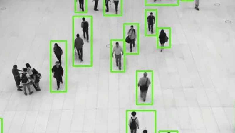
- Motion Detection: In surveillance video, motion detection technology has numerous applications, ranging from indoor and outdoor security environments, traffic control, behaviour detection during sports activities, detection of unattended objects, and even compression of video. In the figure below, see how detecting the movement of people in a video stream could be useful in a surveillance application. Notice how the group of people standing still in the left side of the image are not detected. Only those in motion are captured. Do refer to this paper to study this approach in detail.
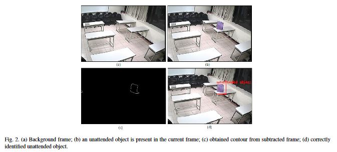
- Unattended object detection: Any unattended object in public places is generally considered as a suspicious object. An effective and safe solution could be: (Unattended Object Detection through Contour Formation using Background Subtraction).
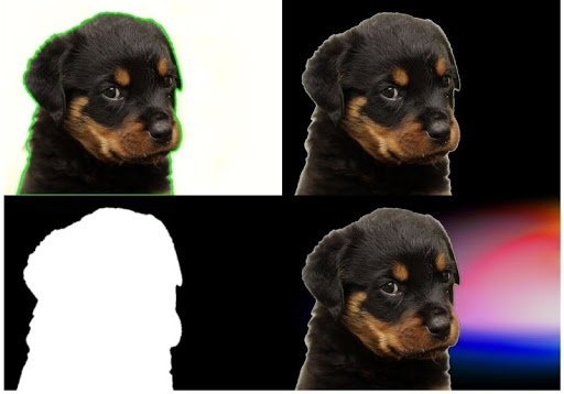
- Background / Foreground Segmentation: To replace the background of an image with another, you need to perform image-foreground extraction (similar to image segmentation). Using contours is one approach that can be used to perform segmentation. Refer to this post for more details. The following images show simple examples of such an application:


What are Contours
When we join all the points on the boundary of an object, we get a contour. Typically, a specific contour refers to boundary pixels that have the same color and intensity. OpenCV makes it really easy to find and draw contours in images. It provides two simple functions:
findContours()drawContours()
Also, it has two different algorithms for contour detection:
CHAIN_APPROX_SIMPLECHAIN_APPROX_NONE
We will cover these in detail, in the examples below. The following figure shows how these algorithms can detect the contours of simple objects.

Now that you have been introduced to contours, let’s discuss the steps involved in their detection.
Steps for Detecting and Drawing Contours in OpenCV
OpenCV makes this a fairly simple task. Just follow these steps:
- Read the Image and convert it to Grayscale Format
Read the image and convert the image to grayscale format. Converting the image to grayscale is very important as it prepares the image for the next step. Converting the image to a single channel grayscale image is important for thresholding, which in turn is necessary for the contour detection algorithm to work properly.
- Apply Binary Thresholding
While finding contours, first always apply binary thresholding or Canny edge detection to the grayscale image. Here, we will apply binary thresholding.
This converts the image to black and white, highlighting the objects-of-interest to make things easy for the contour-detection algorithm. Thresholding turns the border of the object in the image completely white, with all pixels having the same intensity. The algorithm can now detect the borders of the objects from these white pixels.
Note: The black pixels, having value 0, are perceived as background pixels and ignored.
At this point, one question may arise. What if we use single channels like R (red), G (green), or B (blue) instead of grayscale (thresholded) images? In such a case, the contour detection algorithm will not work well. As we discussed previously, the algorithm looks for borders, and similar intensity pixels to detect the contours. A binary image provides this information much better than a single (RGB) color channel image. In a later portion of the blog, we have resultant images when using only a single R, G, or B channel instead of grayscale and thresholded images.
- Find the Contours
Use the findContours() function to detect the contours in the image.
- Draw Contours on the Original RGB Image.
Once contours have been identified, use the drawContours() function to overlay the contours on the original RGB image.
The above steps will make much more sense, and become even clearer when we will start to code.
Finding and Drawing Contours using OpenCV
Start by importing OpenCV, and reading the input image.
Python:
import cv2

# read the image
image = cv2.imread('input/image_1.jpg')

We assume that the image is inside the input folder of the current project directory. The next step is to convert the image into a grayscale image (single channel format).
Note: All the C++ code is contained within the main() function.
C++:
#include<opencv2/opencv.hpp>
#include <iostream>

using namespace std;
using namespace cv;

int main() {
   // read the image
   Mat image = imread("input/image_1.jpg");
Next, use the cvtColor() function to convert the original RGB image to a grayscale image.
Python:
# convert the image to grayscale format
img_gray = cv2.cvtColor(image, cv2.COLOR_BGR2GRAY)
C++:
// convert the image to grayscale format
Mat img_gray;
cvtColor(image, img_gray, COLOR_BGR2GRAY);
Now, use the threshold() function to apply a binary threshold to the image. Any pixel with a value greater than 150 will be set to a value of 255 (white). All remaining pixels in the resulting image will be set to 0 (black). The threshold value of 150 is a tunable parameter, so you can experiment with it.
After thresholding, visualize the binary image, using the imshow() function as shown below.
Python:
# apply binary thresholding
ret, thresh = cv2.threshold(img_gray, 150, 255, cv2.THRESH_BINARY)
# visualize the binary image
cv2.imshow('Binary image', thresh)
cv2.waitKey(0)
cv2.imwrite('image_thres1.jpg', thresh)
cv2.destroyAllWindows()
C++:
// apply binary thresholding
Mat thresh;
threshold(img_gray, thresh, 150, 255, THRESH_BINARY);
imshow("Binary mage", thresh);
waitKey(0);
imwrite("image_thres1.jpg", thresh);
destroyAllWindows();
Check out the image below! It is a binary representation of the original RGB image. You can clearly see how the pen, the borders of the tablet and the phone are all white. The contour algorithm will consider these as objects, and find the contour points around the borders of these white objects.
Note how the background is completely black, including the backside of the phone. Such regions will be ignored by the algorithm. Taking the white pixels around the perimeter of each object as similar-intensity pixels, the algorithm will join them to form a contour based on a similarity measure.

Drawing Contours using CHAIN_APPROX_NONE
Now, let’s find and draw the contours, using the CHAIN_APPROX_NONE method.
Start with the findContours() function. It has three required arguments, as shown below. For optional arguments, please refer to the documentation page here.
image: The binary input image obtained in the previous step.mode: This is the contour-retrieval mode. We provided this asRETR_TREE, which means the algorithm will retrieve all possible contours from the binary image. More contour retrieval modes are available, we will be discussing them too. You can learn more details on these options here.method: This defines the contour-approximation method. In this example, we will useCHAIN_APPROX_NONE.Though slightly slower thanCHAIN_APPROX_SIMPLE, we will use this method here tol store ALL contour points.
It’s worth emphasizing here that mode refers to the type of contours that will be retrieved, while method refers to which points within a contour are stored. We will be discussing both in more detail below.
It is easy to visualize and understand results from different methods on the same image.
In the code samples below, we therefore make a copy of the original image and then demonstrate the methods (not wanting to edit the original).
Next, use the drawContours() function to overlay the contours on the RGB image. This function has four required and several optional arguments. The first four arguments below are required. For the optional arguments, please refer to the documentation page here.
image: This is the input RGB image on which you want to draw the contour.contours: Indicates thecontoursobtained from thefindContours()function.contourIdx: The pixel coordinates of the contour points are listed in the obtained contours. Using this argument, you can specify the index position from this list, indicating exactly which contour point you want to draw. Providing a negative value will draw all the contour points.color: This indicates the color of the contour points you want to draw. We are drawing the points in green.thickness: This is the thickness of contour points.
Python:
# detect the contours on the binary image using cv2.CHAIN_APPROX_NONE
contours, hierarchy = cv2.findContours(image=thresh, mode=cv2.RETR_TREE, method=cv2.CHAIN_APPROX_NONE)

# draw contours on the original image
image_copy = image.copy()
cv2.drawContours(image=image_copy, contours=contours, contourIdx=-1, color=(0, 255, 0), thickness=2, lineType=cv2.LINE_AA)

# see the results
cv2.imshow('None approximation', image_copy)
cv2.waitKey(0)
cv2.imwrite('contours_none_image1.jpg', image_copy)
cv2.destroyAllWindows()
C++:
// detect the contours on the binary image using cv2.CHAIN_APPROX_NONE
vector<vector<Point>> contours;
vector<Vec4i> hierarchy;
findContours(thresh, contours, hierarchy, RETR_TREE, CHAIN_APPROX_NONE);
// draw contours on the original image
Mat image_copy = image.clone();
drawContours(image_copy, contours, -1, Scalar(0, 255, 0), 2);
imshow("None approximation", image_copy);
waitKey(0);
imwrite("contours_none_image1.jpg", image_copy);
destroyAllWindows();
Executing the above code will produce and display the image shown below. We also save the image to disk.

The following figure shows the original image (on the left), as well as the original image with the contours overlaid (on the right).

As you can see in the above figure, the contours produced by the algorithm do a nice job of identifying the boundary of each object. However, if you look closely at the phone, you will find that it contains more than one contour. Separate contours have been identified for the circular areas associated with the camera lens and light. There are also ‘secondary’ contours, along portions of the edge of the phone.
Keep in mind that the accuracy and quality of the contour algorithm is heavily dependent on the quality of the binary image that is supplied (look at the binary image in the previous section again, you can see the lines associated with these secondary contours). Some applications require high quality contours. In such cases, experiment with different thresholds when creating the binary image, and see if that improves the resulting contours.
There are other approaches that can be used to eliminate unwanted contours from the binary maps prior to contour generation. You can also use more advanced features associated with the contour algorithm that we will be discussing here.
Using Single Channel: Red, Green, or Blue
Just to get an idea, the following are some results when using red, green and blue channels separately, while detecting contours. We discussed this in the contour detection steps previously. The following are the Python and C++ code for the same image as above.
Python:
import cv2

# read the image
image = cv2.imread('input/image_1.jpg')

# B, G, R channel splitting
blue, green, red = cv2.split(image)

# detect contours using blue channel and without thresholding
contours1, hierarchy1 = cv2.findContours(image=blue, mode=cv2.RETR_TREE, method=cv2.CHAIN_APPROX_NONE)

# draw contours on the original image
image_contour_blue = image.copy()
cv2.drawContours(image=image_contour_blue, contours=contours1, contourIdx=-1, color=(0, 255, 0), thickness=2, lineType=cv2.LINE_AA)
# see the results
cv2.imshow('Contour detection using blue channels only', image_contour_blue)
cv2.waitKey(0)
cv2.imwrite('blue_channel.jpg', image_contour_blue)
cv2.destroyAllWindows()

# detect contours using green channel and without thresholding
contours2, hierarchy2 = cv2.findContours(image=green, mode=cv2.RETR_TREE, method=cv2.CHAIN_APPROX_NONE)
# draw contours on the original image
image_contour_green = image.copy()
cv2.drawContours(image=image_contour_green, contours=contours2, contourIdx=-1, color=(0, 255, 0), thickness=2, lineType=cv2.LINE_AA)
# see the results
cv2.imshow('Contour detection using green channels only', image_contour_green)
cv2.waitKey(0)
cv2.imwrite('green_channel.jpg', image_contour_green)
cv2.destroyAllWindows()

# detect contours using red channel and without thresholding
contours3, hierarchy3 = cv2.findContours(image=red, mode=cv2.RETR_TREE, method=cv2.CHAIN_APPROX_NONE)
# draw contours on the original image
image_contour_red = image.copy()
cv2.drawContours(image=image_contour_red, contours=contours3, contourIdx=-1, color=(0, 255, 0), thickness=2, lineType=cv2.LINE_AA)
# see the results
cv2.imshow('Contour detection using red channels only', image_contour_red)
cv2.waitKey(0)
cv2.imwrite('red_channel.jpg', image_contour_red)
cv2.destroyAllWindows()
C++:
#include<opencv2/opencv.hpp>
#include <iostream>

using namespace std;
using namespace cv;

int main() {
   // read the image
   Mat image = imread("input/image_1.jpg");

   // B, G, R channel splitting
   Mat channels[3];
   split(image, channels);

   // detect contours using blue channel and without thresholding
   vector<vector<Point>> contours1;
   vector<Vec4i> hierarchy1;
   findContours(channels[0], contours1, hierarchy1, RETR_TREE, CHAIN_APPROX_NONE);
   // draw contours on the original image
   Mat image_contour_blue = image.clone();
   drawContours(image_contour_blue, contours1, -1, Scalar(0, 255, 0), 2);
   imshow("Contour detection using blue channels only", image_contour_blue);
   waitKey(0);
   imwrite("blue_channel.jpg", image_contour_blue);
   destroyAllWindows();

   // detect contours using green channel and without thresholding
   vector<vector<Point>> contours2;
   vector<Vec4i> hierarchy2;
   findContours(channels[1], contours2, hierarchy2, RETR_TREE, CHAIN_APPROX_NONE);
   // draw contours on the original image
   Mat image_contour_green = image.clone();
   drawContours(image_contour_green, contours2, -1, Scalar(0, 255, 0), 2);
   imshow("Contour detection using green channels only", image_contour_green);
   waitKey(0);
   imwrite("green_channel.jpg", image_contour_green);
   destroyAllWindows();

   // detect contours using red channel and without thresholding
   vector<vector<Point>> contours3;
   vector<Vec4i> hierarchy3;
   findContours(channels[2], contours3, hierarchy3, RETR_TREE, CHAIN_APPROX_NONE);
   // draw contours on the original image
   Mat image_contour_red = image.clone();
   drawContours(image_contour_red, contours3, -1, Scalar(0, 255, 0), 2);
   imshow("Contour detection using red channels only", image_contour_red);
   waitKey(0);
   imwrite("red_channel.jpg", image_contour_red);
   destroyAllWindows();
}
The following figure shows the contour detection results for all the three separate color channels.

In the above image we can see that the contour detection algorithm is not able to find the contours properly. This is because it is not able to detect the borders of the objects properly, and also the intensity difference between the pixels is not well defined. This is the reason we prefer to use a grayscale, and binary thresholded image for detecting contours.
Drawing Contours using CHAIN_APPROX_SIMPLE
Let’s find out now how the CHAIN_APPROX_SIMPLE algorithm works and what makes it different from the CHAIN_APPROX_NONE algorithm.
Here’s the code for it:
Python:
"""
Now let's try with `cv2.CHAIN_APPROX_SIMPLE`
"""
# detect the contours on the binary image using cv2.ChAIN_APPROX_SIMPLE
contours1, hierarchy1 = cv2.findContours(thresh, cv2.RETR_TREE, cv2.CHAIN_APPROX_SIMPLE)
# draw contours on the original image for `CHAIN_APPROX_SIMPLE`
image_copy1 = image.copy()
cv2.drawContours(image_copy1, contours1, -1, (0, 255, 0), 2, cv2.LINE_AA)
# see the results
cv2.imshow('Simple approximation', image_copy1)
cv2.waitKey(0)
cv2.imwrite('contours_simple_image1.jpg', image_copy1)
cv2.destroyAllWindows()
C++:
// Now let us try with CHAIN_APPROX_SIMPLE`
// detect the contours on the binary image using cv2.CHAIN_APPROX_NONE
vector<vector<Point>> contours1;
vector<Vec4i> hierarchy1;
findContours(thresh, contours1, hierarchy1, RETR_TREE, CHAIN_APPROX_SIMPLE);
// draw contours on the original image
Mat image_copy1 = image.clone();
drawContours(image_copy1, contours1, -1, Scalar(0, 255, 0), 2);
imshow("Simple approximation", image_copy1);
waitKey(0);
imwrite("contours_simple_image1.jpg", image_copy1);
destroyAllWindows();
The only difference here is that we specify the method for findContours() as CHAIN_APPROX_SIMPLE instead of CHAIN_APPROX_NONE.
The CHAIN_APPROX_SIMPLE algorithm compresses horizontal, vertical, and diagonal segments along the contour and leaves only their end points. This means that any of the points along the straight paths will be dismissed, and we will be left with only the end points. For example, consider a contour, along a rectangle. All the contour points, except the four corner points will be dismissed. This method is faster than the CHAIN_APPROX_NONE because the algorithm does not store all the points, uses less memory, and therefore, takes less time to execute.
The following image shows the results.

If you observe closely, there are almost no differences between the outputs of CHAIN_APPROX_NONE and CHAIN_APPROX_SIMPLE.
Now, why is that?
The credit goes to the drawContours() function. Although the CHAIN_APPROX_SIMPLE method typically results in fewer points, the drawContours() function automatically connects adjacent points, joining them even if they are not in the contours list.
So, how do we confirm that the CHAIN_APPROX_SIMPLE algorithm is actually working?
- The most straightforward way is to loop over the contour points manually, and draw a circle on the detected contour coordinates, using OpenCV.
- Also, we use a different image that will actually help us visualize the results of the algorithm.
The following code uses the above image to visualize the effect of the CHAIN_APPROX_SIMPLE algorithm. Almost everything is the same as in the previous code example, except the two additional for loops and some variable names.
- The first
forloop cycles over each contour area present in thecontourslist. - The second loops over each of the coordinates in that area.
- We then draw a green circle on each coordinate point, using the
circle()function from OpenCV. - Finally, we visualize the results and save it to disk.
Python:
# to actually visualize the effect of `CHAIN_APPROX_SIMPLE`, we need a proper image
image1 = cv2.imread('input/image_2.jpg')
img_gray1 = cv2.cvtColor(image1, cv2.COLOR_BGR2GRAY)

ret, thresh1 = cv2.threshold(img_gray1, 150, 255, cv2.THRESH_BINARY)
contours2, hierarchy2 = cv2.findContours(thresh1, cv2.RETR_TREE,
                                               cv2.CHAIN_APPROX_SIMPLE)
image_copy2 = image1.copy()
cv2.drawContours(image_copy2, contours2, -1, (0, 255, 0), 2, cv2.LINE_AA)
cv2.imshow('SIMPLE Approximation contours', image_copy2)
cv2.waitKey(0)
image_copy3 = image1.copy()
for i, contour in enumerate(contours2): # loop over one contour area
   for j, contour_point in enumerate(contour): # loop over the points
       # draw a circle on the current contour coordinate
       cv2.circle(image_copy3, ((contour_point[0][0], contour_point[0][1])), 2, (0, 255, 0), 2, cv2.LINE_AA)
# see the results
cv2.imshow('CHAIN_APPROX_SIMPLE Point only', image_copy3)
cv2.waitKey(0)
cv2.imwrite('contour_point_simple.jpg', image_copy3)
cv2.destroyAllWindows()
C++:
// using a proper image for visualizing CHAIN_APPROX_SIMPLE
Mat image1 = imread("input/image_2.jpg");
Mat img_gray1;
cvtColor(image1, img_gray1, COLOR_BGR2GRAY);
Mat thresh1;
threshold(img_gray1, thresh1, 150, 255, THRESH_BINARY);
vector<vector<Point>> contours2;
vector<Vec4i> hierarchy2;
findContours(thresh1, contours2, hierarchy2, RETR_TREE, CHAIN_APPROX_NONE);
Mat image_copy2 = image1.clone();
drawContours(image_copy2, contours2, -1, Scalar(0, 255, 0), 2);
imshow("None approximation", image_copy2);
waitKey(0);
imwrite("contours_none_image1.jpg", image_copy2);
destroyAllWindows();
Mat image_copy3 = image1.clone();
for(int i=0; i<contours2.size(); i=i+1){
   for (int j=0; j<contours2[i].size(); j=j+1){
       circle(image_copy3, (contours2[i][0], contours2[i][1]), 2, Scalar(0, 255, 0), 2);
       }
   }
   imshow("CHAIN_APPROX_SIMPLE Point only", image_copy3);
   waitKey(0);
   imwrite("contour_point_simple.jpg", image_copy3);
   destroyAllWindows();
Executing the code above, produces the following result:
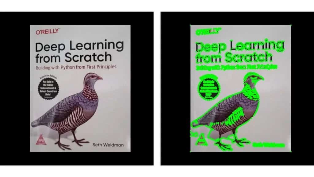
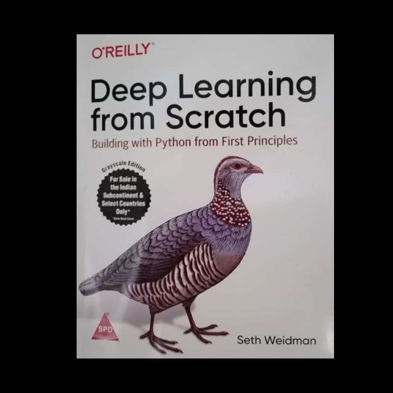
Observe the output image, which is on the right-hand side in the above figure. Note that the vertical and horizontal sides of the book contain only four points at the corners of the book. Also observe that the letters and bird are indicated with discrete points and not line segments.
Contour Hierarchies
Hierarchies denote the parent-child relationship between contours. You will see how each contour-retrieval mode affects contour detection in images, and produces hierarchical results.
Parent-Child Relationship
Objects detected by contour-detection algorithms in an image could be:
- Single objects scattered around in an image (as in the first example), or
- Objects and shapes inside one another
In most cases, where a shape contains more shapes, we can safely conclude that the outer shape is a parent of the inner shape.
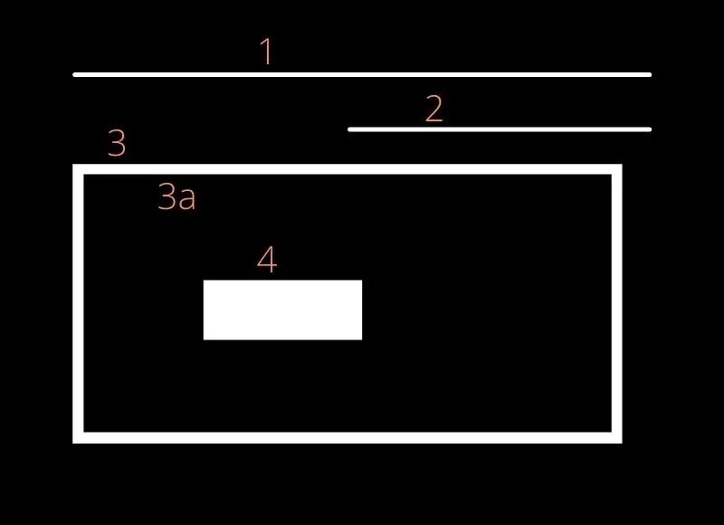
Take a look at the following figure, it contains several simple shapes that will help demonstrate contour hierarchies.

Now see below figure, where the contours associated with each shape in Figure 10 have been identified. Each of the numbers in Figure 11 have a significance.
- All the individual numbers, i.e., 1, 2, 3, and 4 are separate objects, according to the contour hierarchy and parent-child relationship.
- We can say that the 3a is a child of 3. Note that 3a represents the interior portion of contour 3.
- Contours 1, 2, and 4 are all parent shapes, without any associated child, and their numbering is thus arbitrary. In other words, contour 2 could have been labeled as 1 and vice-versa.
Contour Relationship Representation
You’ve seen that the findContours() function returns two outputs: The contours list, and the hierarchy. Let’s now understand the contour hierarchy output in detail.
The contour hierarchy is represented as an array, which in turn contains arrays of four values. It is represented as:
[Next, Previous, First_Child, Parent]
So, what do all these values mean?
Next: Denotes the next contour in an image, which is at the same hierarchical level. So,
- For contour 1, the next contour at the same hierarchical level is 2. Here,
Nextwill be 2. - Accordingly, contour 3 has no contour at the same hierarchical level as itself. So, it’s
Nextvalue will be -1.
Previous: Denotes the previous contour at the same hierarchical level. This means that contour 1 will always have its Previous value as -1.
First_Child: Denotes the first child contour of the contour we are currently considering.
- Contours 1 and 2 have no children at all. So, the index values for their
First_Childwill be -1. - But contour 3 has a child. So, for contour 3, the
First_Childposition value will be the index position of 3a.
Parent: Denotes the parent contour’s index position for the current contour.
- Contours 1 and 2, as is obvious, do not have any
Parentcontour. - For the contour 3a, its
Parentis going to be contour 3 - For contour 4, the parent is contour 3a
The above explanations make sense, but how do we actually visualize these hierarchy arrays? The best way is to:
- Use a simple image with lines and shapes like the previous image
- Detect the contours and hierarchies, using different retrieval modes
- Then print the values to visualize them
Different Contour Retrieval Techniques
Thus far, we used one specific retrieval technique, RETR_TREE to find and draw contours, but there are three more contour-retrieval techniques in OpenCV, namely, RETR_LIST, RETR_EXTERNAL and RETR_CCOMP.
So let’s now use the image in Figure 10 to review each of these four methods, along with their associated code to get the contours.
The following code reads the image from disk, converts it to grayscale, and applies binary thresholding.
Python:
"""
Contour detection and drawing using different extraction modes to complement
the understanding of hierarchies
"""
image2 = cv2.imread('input/custom_colors.jpg')
img_gray2 = cv2.cvtColor(image2, cv2.COLOR_BGR2GRAY)
ret, thresh2 = cv2.threshold(img_gray2, 150, 255, cv2.THRESH_BINARY)
C++:
/*
Contour detection and drawing using different extraction modes to complement the understanding of hierarchies
*/
Mat image2 = imread("input/custom_colors.jpg");
Mat img_gray2;
cvtColor(image2, img_gray2, COLOR_BGR2GRAY);
Mat thresh2;
threshold(img_gray2, thresh2, 150, 255, THRESH_BINARY);
RETR_LIST
The RETR_LIST contour retrieval method does not create any parent child relationship between the extracted contours. So, for all the contour areas that are detected, the First_Child and Parent index position values are always -1.
All the contours will have their corresponding Previous and Next contours as discussed above.
See how the RETR_LIST method is implemented in code.
Python:
contours3, hierarchy3 = cv2.findContours(thresh2, cv2.RETR_LIST, cv2.CHAIN_APPROX_NONE)
image_copy4 = image2.copy()
cv2.drawContours(image_copy4, contours3, -1, (0, 255, 0), 2, cv2.LINE_AA)
# see the results
cv2.imshow('LIST', image_copy4)
print(f"LIST: {hierarchy3}")
cv2.waitKey(0)
cv2.imwrite('contours_retr_list.jpg', image_copy4)
cv2.destroyAllWindows()
C++:
vector<vector<Point>> contours3;
vector<Vec4i> hierarchy3;
findContours(thresh2, contours3, hierarchy3, RETR_LIST, CHAIN_APPROX_NONE);
Mat image_copy4 = image2.clone();
drawContours(image_copy4, contours3, -1, Scalar(0, 255, 0), 2);
imshow("LIST", image_copy4);
waitKey(0);
imwrite("contours_retr_list.jpg", image_copy4);
destroyAllWindows();
Executing the above code produces the following output:
LIST: [[[ 1 -1 -1 -1]
[ 2  0 -1 -1]
[ 3  1 -1 -1]
[ 4  2 -1 -1]
[-1  3 -1 -1]]]
You can clearly see that the 3rd and 4th index positions of all the detected contour areas are -1, as expected.
RETR_EXTERNAL
The RETR_EXTERNAL contour retrieval method is a really interesting one. It only detects the parent contours, and ignores any child contours. So, all the inner contours like 3a and 4 will not have any points drawn on them.
Python:
contours4, hierarchy4 = cv2.findContours(thresh2, cv2.RETR_EXTERNAL, cv2.CHAIN_APPROX_NONE)
image_copy5 = image2.copy()
cv2.drawContours(image_copy5, contours4, -1, (0, 255, 0), 2, cv2.LINE_AA)
# see the results
cv2.imshow('EXTERNAL', image_copy5)
print(f"EXTERNAL: {hierarchy4}")
cv2.waitKey(0)
cv2.imwrite('contours_retr_external.jpg', image_copy5)
cv2.destroyAllWindows()
C++:
vector<vector<Point>> contours4;
vector<Vec4i> hierarchy4;
findContours(thresh2, contours4, hierarchy4, RETR_EXTERNAL, CHAIN_APPROX_NONE);
Mat image_copy5 = image2.clone();
drawContours(image_copy5, contours4, -1, Scalar(0, 255, 0), 2);
imshow("EXTERNAL", image_copy5);
waitKey(0);
imwrite("contours_retr_external.jpg", image_copy4);
destroyAllWindows();
The above code produces the following output:
EXTERNAL: [[[ 1 -1 -1 -1]
[ 2  0 -1 -1]
[-1  1 -1 -1]]]

The above output image shows only the points drawn on contours 1, 2, and 3. Contours 3a and 4 are omitted as they are child contours.
RETR_CCOMP
Unlike RETR_EXTERNAL,RETR_CCOMP retrieves all the contours in an image. Along with that, it also applies a 2-level hierarchy to all the shapes or objects in the image.
This means:
- All the outer contours will have hierarchy level 1
- All the inner contours will have hierarchy level 2
But what if we have a contour inside another contour with hierarchy level 2? Just like we have contour 4 after contour 3a.
In that case:
- Again, contour 4 will have hierarchy level 1.
- If there are any contours inside contour 4, they will have hierarchy level 2.
In the following image, the contours have been numbered according to their hierarchy level, as explained above.
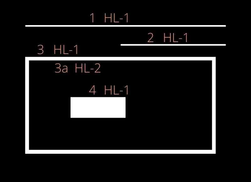
The above image shows the hierarchy level as HL-1 or HL-2 for levels 1 and 2 respectively. Now, let us take a look at the code and the output hierarchy array also.
Python:
contours5, hierarchy5 = cv2.findContours(thresh2, cv2.RETR_CCOMP, cv2.CHAIN_APPROX_NONE)
image_copy6 = image2.copy()
cv2.drawContours(image_copy6, contours5, -1, (0, 255, 0), 2, cv2.LINE_AA)

# see the results
cv2.imshow('CCOMP', image_copy6)
print(f"CCOMP: {hierarchy5}")
cv2.waitKey(0)
cv2.imwrite('contours_retr_ccomp.jpg', image_copy6)
cv2.destroyAllWindows()
C++:
vector<vector<Point>> contours5;
vector<Vec4i> hierarchy5;
findContours(thresh2, contours5, hierarchy5, RETR_CCOMP, CHAIN_APPROX_NONE);
Mat image_copy6 = image2.clone();
drawContours(image_copy6, contours5, -1, Scalar(0, 255, 0), 2);
imshow("EXTERNAL", image_copy6);
// cout << "EXTERNAL:" << hierarchy5;
waitKey(0);
imwrite("contours_retr_ccomp.jpg", image_copy6);
destroyAllWindows();
Executing the above code produces the following output:
CCOMP: [[[ 1 -1 -1 -1]
[ 3  0  2 -1]
[-1 -1 -1  1]
[ 4  1 -1 -1]
[-1  3 -1 -1]]]
Here, we see that all the Next, Previous, First_Child, and Parent relationships are maintained, according to the contour-retrieval method, as all the contours are detected. As expected, the Previous of the first contour area is -1. And the contours which do not have any Parent, also have the value -1
RETR_TREE
Just like RETR_CCOMP, RETR_TREE also retrieves all the contours. It also creates a complete hierarchy, with the levels not restricted to 1 or 2. Each contour can have its own hierarchy, in line with the level it is on, and the corresponding parent-child relationship that it has.

From the above figure, it is clear that:
- Contours 1, 2, and 3 are at the same level, that is level 0.
- Contour 3a is present at hierarchy level 1, as it is a child of contour 3.
- Contour 4 is a new contour area, so its hierarchy level is 2.
The following code uses RETR_TREE mode to retrieve contours.
Python:
contours6, hierarchy6 = cv2.findContours(thresh2, cv2.RETR_TREE, cv2.CHAIN_APPROX_NONE)
image_copy7 = image2.copy()
cv2.drawContours(image_copy7, contours6, -1, (0, 255, 0), 2, cv2.LINE_AA)
# see the results
cv2.imshow('TREE', image_copy7)
print(f"TREE: {hierarchy6}")
cv2.waitKey(0)
cv2.imwrite('contours_retr_tree.jpg', image_copy7)
cv2.destroyAllWindows()
C++:
vector<vector<Point>> contours6;
vector<Vec4i> hierarchy6;
findContours(thresh2, contours6, hierarchy6, RETR_TREE, CHAIN_APPROX_NONE);
Mat image_copy7 = image2.clone();
drawContours(image_copy7, contours6, -1, Scalar(0, 255, 0), 2);
imshow("EXTERNAL", image_copy7);
// cout << "EXTERNAL:" << hierarchy6;
waitKey(0);
imwrite("contours_retr_tree.jpg", image_copy7);
destroyAllWindows();
Executing the above code produces the following output:
TREE: [[[ 3 -1  1 -1]
[-1 -1  2  0]
[-1 -1 -1  1]
[ 4  0 -1 -1]
[-1  3 -1 -1]]]
Finally, let’s look at the complete image with all the contours drawn when using RETR_TREE mode.
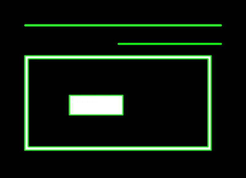
All the contours are drawn as expected, and the contour areas are clearly visible. You also infer that contours 3 and 3a are two separate contours, as they have different contour boundaries and areas. At the same time, it is very evident that contour 3a is a child of contour 3.
Now that you are familiar with all the contour algorithms available in OpenCV, along with their respective input parameters and configurations, go experiment and see for yourself how they work.
A Run Time Comparison of Different Contour Retrieval Methods
It’s not enough to know the contour-retrieval methods. You should also be aware of their relative processing time. The following table compares the runtime for each method discussed above.
| Contour Retrieval Method | Time Take (in seconds) |
| RETR_LIST | 0.000382 |
| RETR_EXTERNAL | 0.000554 |
| RETR_CCOMP | 0.001845 |
| RETR_TREE | 0.005594 |
Some interesting conclusions emerge from the above table:
RETR_LISTandRETR_EXTERNALtake the least amount of time to execute, sinceRETR_LISTdoes not define any hierarchy andRETR_EXTERNALonly retrieves the parent contoursRETR_CCOMPtakes the second highest time to execute. It retrieves all the contours and defines a two-level hierarchy.RETR_TREEtakes the maximum time to execute for it retrieves all the contours, and defines the independent hierarchy level for each parent-child relationship as well.
Although the above times may not seem significant, it is important to be aware of the differences for applications that may require a significant amount of contour processing. It is also worth noting that this processing time may vary, depending to an extent on the contours they extract, and the hierarchy levels they define.
Limitations
So far, all the examples we explored seemed interesting, and their results encouraging. However, there are cases where the contour algorithm might fail to deliver meaningful and useful results. Let’s consider such an example too.
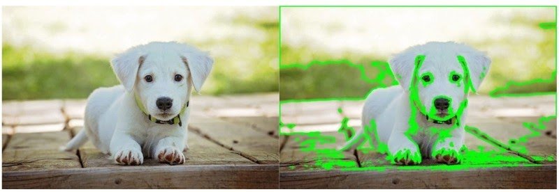
- When the objects in an image are strongly contrasted against their background, you can clearly identify the contours associated with each object. But what if you have an image, like Figure 16 below. It not only has a bright object (puppy), but also a background cluttered with the same value (brightness) as the object of interest (puppy). You find that the contours in the right-hand image are not even complete. Also, there are multiple unwanted contours standing out in the background area.
- Contour detection can also fail, when the background of the object in the image is full of lines.
Taking Your Learning Further
If you think that you have learned something interesting in this article and would like to expand your knowledge, then you may like the Computer Vision 1 course offered by OpenCV. This is a great course to get started with OpenCV and Computer Vision which will be very hands-on and perfect to get you started and up to speed with OpenCV. The best part, you can take it in either Python or C++, whichever you choose. You can visit the course page here to know more about it.
Summary
You started with contour detection, and learned to implement that in OpenCV. Saw how applications use contours for mobility detection and segmentation. Next, we demonstrated the use of four different retrieval modes and two contour-approximation methods. You also learned to draw contours. We concluded with a discussion of contour hierarchies, and how different contour-retrieval modes affect the drawing of contours on an image.
Key takeaways:
- The contour-detection algorithms in OpenCV work very well, when the image has a dark background and a well-defined object-of-interest.
- But when the background of the input image is cluttered or has the same pixel intensity as the object-of-interest, the algorithms don’t fare so well.
You have all the code here, why not experiment with different images now! Try images containing varied shapes, and experiment with different threshold values. Also, explore different retrieval modes, using test images that contain nested contours. This way, you can fully appreciate the hierarchical relationships between objects.
100K+ Learners
Join Free OpenCV Bootcamp3 Hours of Learning