


Edge detection is an image-processing technique that is used to identify the boundaries (edges) of objects or regions within an image. Edges are among the most important features associated with images. We know the underlying structure of an image through its edges. Computer vision processing pipelines, therefore, extensively use edge detection in applications.
How are Edges Detected?
Sudden changes in pixel intensity characterize edges. We need to look for such changes in the neighboring pixels to detect edges. Let’s explore using two important edge-detection algorithms available in OpenCV: Sobel Edge Detection and Canny Edge Detection. We will discuss the theory as well as demonstrate the use of each in OpenCV.
First, take a look at the code that will demonstrate edge detection. Each line of code will be discussed in detail so that you understand it fully.
Python:
import cv2

# Read the original image
img = cv2.imread('test.jpg')
# Display original image
cv2.imshow('Original', img)
cv2.waitKey(0)

# Convert to graycsale
img_gray = cv2.cvtColor(img, cv2.COLOR_BGR2GRAY)
# Blur the image for better edge detection
img_blur = cv2.GaussianBlur(img_gray, (3,3), 0)

# Sobel Edge Detection
sobelx = cv2.Sobel(src=img_blur, ddepth=cv2.CV_64F, dx=1, dy=0, ksize=5) # Sobel Edge Detection on the X axis
sobely = cv2.Sobel(src=img_blur, ddepth=cv2.CV_64F, dx=0, dy=1, ksize=5) # Sobel Edge Detection on the Y axis
sobelxy = cv2.Sobel(src=img_blur, ddepth=cv2.CV_64F, dx=1, dy=1, ksize=5) # Combined X and Y Sobel Edge Detection
# Display Sobel Edge Detection Images
cv2.imshow('Sobel X', sobelx)
cv2.waitKey(0)
cv2.imshow('Sobel Y', sobely)
cv2.waitKey(0)
cv2.imshow('Sobel X Y using Sobel() function', sobelxy)
cv2.waitKey(0)

# Canny Edge Detection
edges = cv2.Canny(image=img_blur, threshold1=100, threshold2=200) # Canny Edge Detection
# Display Canny Edge Detection Image
cv2.imshow('Canny Edge Detection', edges)
cv2.waitKey(0)

cv2.destroyAllWindows()
C++:
#include <opencv2/opencv.hpp>
#include <iostream>
// using namespaces to nullify use of cv::function(); syntax and std::function();
using namespace std;
using namespace cv;

int main()
{
    // Reading image
    Mat img = imread("test.jpg");
    // Display original image
    imshow("original Image", img);
    waitKey(0);

    // Convert to graycsale
    Mat img_gray;
    cvtColor(img, img_gray, COLOR_BGR2GRAY);
    // Blur the image for better edge detection
    Mat img_blur;
    GaussianBlur(img_gray, img_blur, Size(3,3), 0);

    // Sobel edge detection
    Mat sobelx, sobely, sobelxy;
    Sobel(img_blur, sobelx, CV_64F, 1, 0, 5);
    Sobel(img_blur, sobely, CV_64F, 0, 1, 5);
    Sobel(img_blur, sobelxy, CV_64F, 1, 1, 5);
    // Display Sobel edge detection images
    imshow("Sobel X", sobelx);
    waitKey(0);
    imshow("Sobel Y", sobely);
    waitKey(0);
    imshow("Sobel XY using Sobel() function", sobelxy);
    waitKey(0);

    // Canny edge detection
    Mat edges;
    Canny(img_blur, edges, 100, 200, 3, false);
    // Display canny edge detected image
    imshow("Canny edge detection", edges);
    waitKey(0);

    destroyAllWindows();
    return 0;
}


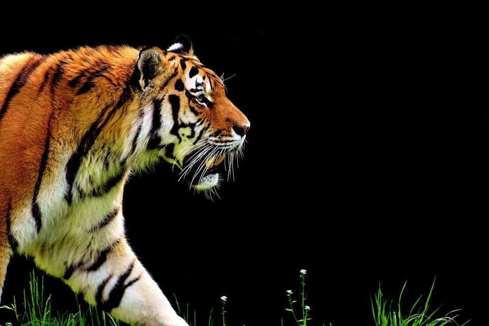
This tiger image will be used for all the examples here.
Before going into each algorithm in detail, let’s complete some preliminary steps for edge detection. Start by importing the OpenCV library, as shown in the code below.
Python:
import cv2

C++:
#include<opencv2/opencv.hpp>
#include<iostream>

// Namespace nullifies the use of cv::function();
using namespace std;
using namespace cv;
The first step is to read in the image, using the imread() function in OpenCV.
Here, we read in the color image as a grayscale image because you do not need color information to detect edges. To learn more refer: Read, Display and Write an Image using OpenCV.
After reading the image, we also blur it, using the GaussianBlur() function. This is done to reduce the noise in the image. In edge detection, numerical derivatives of the pixel intensities have to be computed, and this typically results in ‘noisy’ edges. In other words, the intensity of neighboring pixels in an image (especially near edges) can fluctuate quite a bit, giving rise to edges that don’t represent the predominant edge structure we are looking for.
Blurring smoothens the intensity variation near the edges, making it easier to identify the predominant edge structure within the image. You can refer to the OpenCV documentation for more details on the GaussianBlur() function. We supply the size of the convolution kernel (in this case, 1 3×3 kernel), which specifies the degree of blurring.
Python:
# Read the original image
img = cv2.imread('test.jpg',flags=0)
# Blur the image for better edge detection
img_blur = cv2.GaussianBlur(img,(3,3), SigmaX=0, SigmaY=0)
C++:
// Reading image
Mat img = imread("test.jpg",0);
// Blur the image for better edge detection
Mat img_blur;
GaussianBlur(img, img_blur, Size(3,3), SigmaX=0, SigmaY=0);
Sobel Edge Detection
Sobel Edge Detection is one of the most widely used algorithms for edge detection. The Sobel Operator detects edges marked by sudden changes in pixel intensity, as shown in the figure below.
The rise in intensity is even more evident when we plot the first derivative of the intensity function.
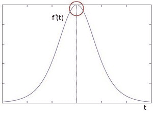
The above plot demonstrates that edges can be detected in areas where the gradient is higher than a particular threshold value. In addition, a sudden change in the derivative will also reveal a change in the pixel intensity. With this in mind, we can approximate the derivative using a 3×3 kernel. We use one kernel to detect sudden changes in pixel intensity in the X direction and another in the Y direction. (To learn more, check this post on image filtering and convolution kernels.
These are the kernels used for Sobel Edge Detection:
(1) 
X-Direction Kernel
(2) 
Y-Direction Kernel
When these kernels are convolved with the original image, you get a ‘Sobel edge image’.
- If we use only the Vertical Kernel, the convolution yields a Sobel image, with edges enhanced in the X-direction
- Using the Horizontal Kernel yields a Sobel image, with edges enhanced in the Y-direction.
Let  and
and  represent the intensity gradient in the
  and
and  directions respectively. If
  and
and  denote the X and Y kernels defined above:
(3) 
(4) 
where  denotes the convolution operator, and
  represents the input image.
The final approximation of the gradient magnitude,  can be computed as:
(5) 
And the orientation of the gradient can then be approximated as:
(6) 
In the code example below, we use the Sobel() function to compute:
- the Sobel edge image individually, in both directions (x and y),
- the composite gradient in both directions (xy)
The following is the syntax for applying Sobel edge detection using OpenCV:
Sobel(src, ddepth, dx, dy)
The parameter ddepth specifies the precision of the output image, while dx and dy specify the order of the derivative in each direction. For example:
- If
dx=1anddy=0, we compute the 1st derivative Sobel image in the x-direction.
If both dx=1 and dy=1, we compute the 1st derivative Sobel image in both directions
Python:
# Sobel Edge Detection
sobelx = cv2.Sobel(src=img_blur, ddepth=cv2.CV_64F, dx=1, dy=0, ksize=5) # Sobel Edge Detection on the X axis
sobely = cv2.Sobel(src=img_blur, ddepth=cv2.CV_64F, dx=0, dy=1, ksize=5) # Sobel Edge Detection on the Y axis
sobelxy = cv2.Sobel(src=img_blur, ddepth=cv2.CV_64F, dx=1, dy=1, ksize=5) # Combined X and Y Sobel Edge Detection

# Display Sobel Edge Detection Images
cv2.imshow('Sobel X', sobelx)
cv2.waitKey(0)

cv2.imshow('Sobel Y', sobely)
cv2.waitKey(0)

cv2.imshow('Sobel X Y using Sobel() function', sobelxy)
cv2.waitKey(0)
C++:
// Sobel edge detection
Mat sobelx, sobely, sobelxy;
Sobel(img_blur, sobelx, CV_64F, 1, 0, 5);
Sobel(img_blur, sobely, CV_64F, 0, 1, 5);
Sobel(img_blur, sobelxy, CV_64F, 1, 1, 5);

// Display Sobel edge detection images
imshow("Sobel X", sobelx);
waitKey(0);
imshow("Sobel Y", sobely);
waitKey(0);
imshow("Sobel XY using Sobel() function", sobelxy);
waitKey(0);
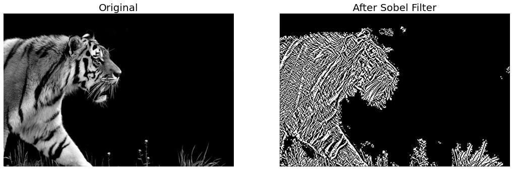
The results are shown in the figures below. See how the Sobel image in the x-direction predominantly identifies vertical edges (i.e. those whose gradient is largest in the x-direction, horizontal). And that in the y-direction identifies horizontal edges (i.e. those whose gradient is largest in the y-direction, vertical). Look closely at the tiger’s stripes in both images. Note how the strong vertical edges of the stripes are more evident in the Sobel image in the x-direction.
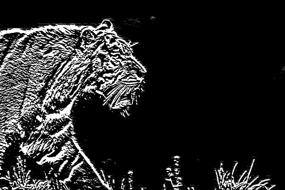
The figure below shows the Sobel image for the gradient in both directions, which distills the original image into an edge structure representation, such that its structural integrity remains intact.

Canny Edge Detection
Canny Edge Detection is one of the most popular edge-detection methods in use today because it is so robust and flexible. The algorithm itself follows a three-stage process for extracting edges from an image. Add to it image blurring, a necessary preprocessing step to reduce noise. This makes it a four-stage process, which includes:
- Noise Reduction
- Calculating the Intensity Gradient of the Image
- Suppression of False Edges
- Hysteresis Thresholding
Noise Reduction
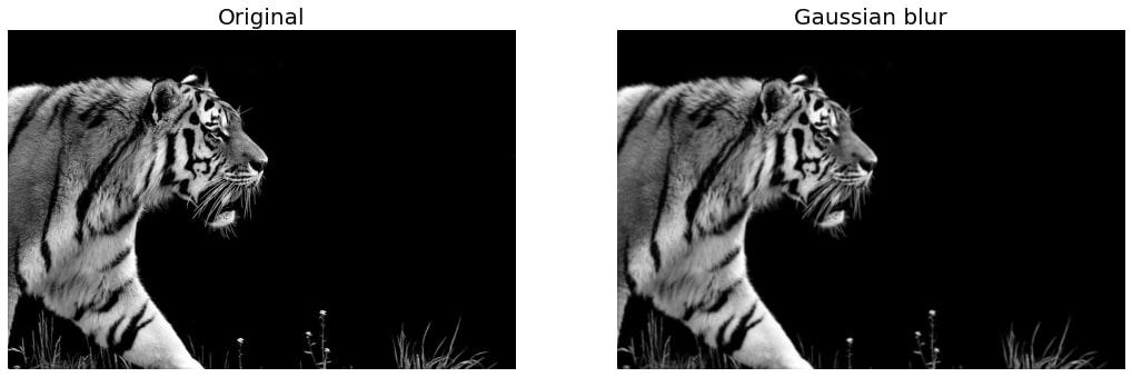
Raw image pixels can often lead to noisy edges, so it is essential to reduce noise before computing edges In Canny Edge Detection, a Gaussian blur filter is used to essentially remove or minimize unnecessary detail that could lead to undesirable edges. Have a look at the tiger in the two images below; Gaussian blur has been applied to the image to the right. As you can see, it appears slightly blurred but still retains a significant amount of detail from which edges can be computed. Click on this link to learn more about blurring.
Calculating the Intensity Gradient of the Image
Once the image has been smoothed (blurred), it is filtered with a Sobel kernel, both horizontally and vertically. The results from these filtering operations are then used to calculate both the intensity gradient magnitude (), and the direction ( ) for each pixel, as shown below.
(7) 
(8) 
The gradient direction is then rounded to the nearest 45-degree angle. The figure below (right) shows the result of this combined processing step.
Suppression of False Edges
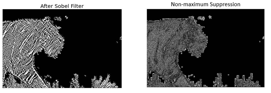
After reducing noise and calculating the intensity gradient, the algorithm in this step uses a technique called non-maximum suppression of edges to filter out unwanted pixels (which may not actually constitute an edge). To accomplish this, each pixel is compared to its neighboring pixels in the positive and negative gradient direction. If the gradient magnitude of the current pixel is greater than its neighboring pixels, it is left unchanged. Otherwise, the magnitude of the current pixel is set to zero. The following image illustrates an example. As you can see, numerous ‘edges’ associated with the tiger’s fur have been significantly subdued.
Hysteresis Thresholding – Edge Detection Using OpenCV
In this final step of Canny Edge Detection, the gradient magnitudes are compared with two threshold values, one smaller than the other.
- If the gradient magnitude value is higher than the larger threshold value, those pixels are associated with solid edges and are included in the final edge map.
- If the gradient magnitude values are lower than the smaller threshold value, the pixels are suppressed and excluded from the final edge map.
- All the other pixels, whose gradient magnitudes fall between these two thresholds, are marked as ‘weak’ edges (i.e. they become candidates for being included in the final edge map).
- If the ‘weak’ pixels are connected to those associated with solid edges, they are also included in the final edge map.
The following is the syntax for applying Canny edge detection using OpenCV:
Canny(image, threshold1, threshold2)
In the code example below, the Canny() function implements the methodology described above. We supply the two thresholds used by the Canny Edge Detection algorithm, and OpenCV handles all the implementation details. Don’t forget to blur the image before calling the Canny() function. It is a highly-recommended preprocessing step. To learn more about the optional arguments, please refer to the OpenCV documentation page.
Python:
# Canny Edge Detection
edges = cv2.Canny(image=img_blur, threshold1=100, threshold2=200)

# Display Canny Edge Detection Image
cv2.imshow('Canny Edge Detection', edges)
cv2.waitKey(0)
C++:
// Canny edge detection
Mat edges;
Canny(img_blur, edges, 100, 200, 3, false);
// Display canny edge detected image
imshow("Canny edge detection", edges);
waitKey(0);
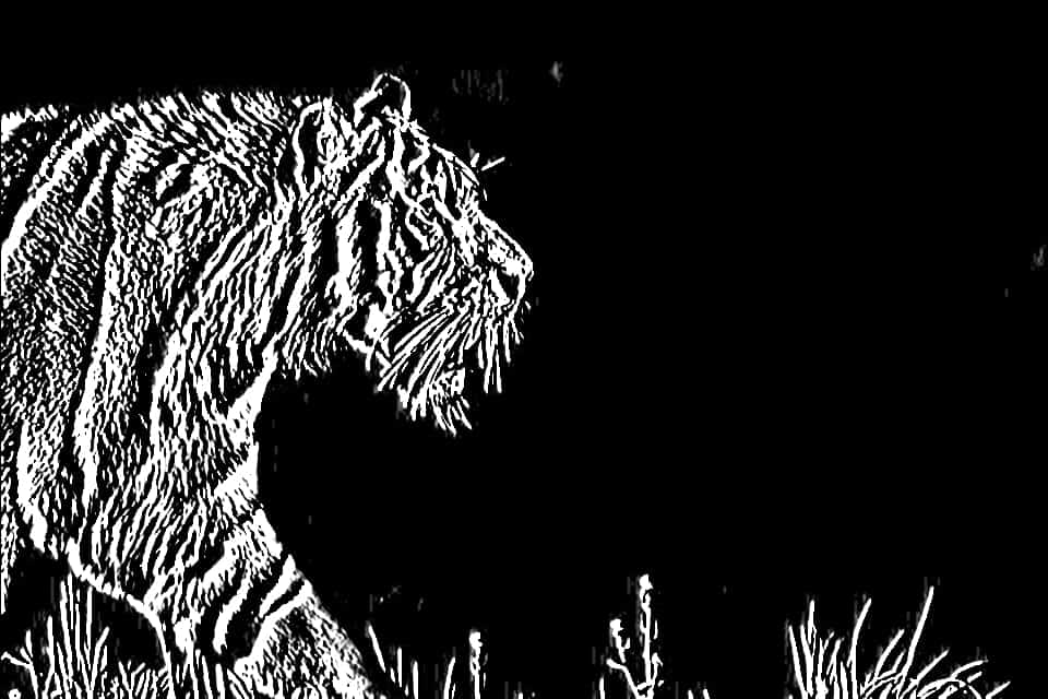
Here are the final results: We use a lower threshold of 100, and an upper threshold of 200. As you can see, the algorithm has identified the predominant edges in the image, eliminating in the process those less important to the overall structure. However, the results can easily be adjusted, so experiment with different images, vary the amount of blurring, and try different threshold values to get a feel for things yourself.
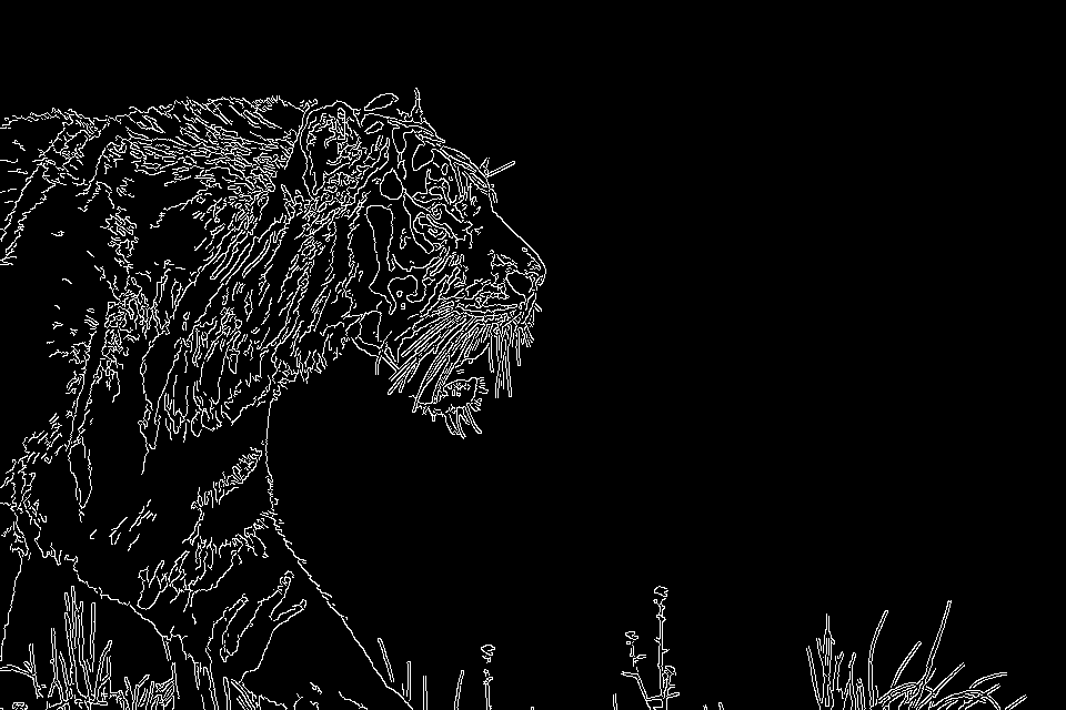
Regarding performance, Canny Edge Detection produces the best results because it uses not only Sobel Edge Detection but also Non-Maximum Suppression and Hysteresis Thresholding. This provides more flexibility in how edges are identified and connected in the final stages of the algorithm.
Summary
We discussed what makes edge detection an important image-processing technique and focused on knowing its two most important algorithms (Sobel Edge Detection and Canny Edge Detection). While demonstrating their use in OpenCV, we highlighted why blurring is an important preprocessing step.
You also saw how Canny Edge Detection actually uses the Sobel operator to compute numerical derivatives. And is robust and flexible, using even Non-Maximum Suppression and Hysteresis Thresholding to maximum advantage. Finally, you understood why Canny Edge Detection is the preferred and most widely used method for performing edge detection.
You can find all the codes discussed in this post at this link →Edge Detection Using OpenCV Colab Notebook.
100K+ Learners
Join Free OpenCV Bootcamp3 Hours of Learning