


In this post, we’re going to provide a 30,000-Foot view of neural networks that’s aimed at absolute beginners who are looking to enter the field of Machine Learning and Deep Learning. In this tutorial, we will simplify many details so that you can grasp the most basic concepts.
- Neural Networks as Black Box
- Understanding the Neural Network Output
- Understanding the Neural Network Input
- What does it mean to train a Neural Network?
Neural Networks as Black Box
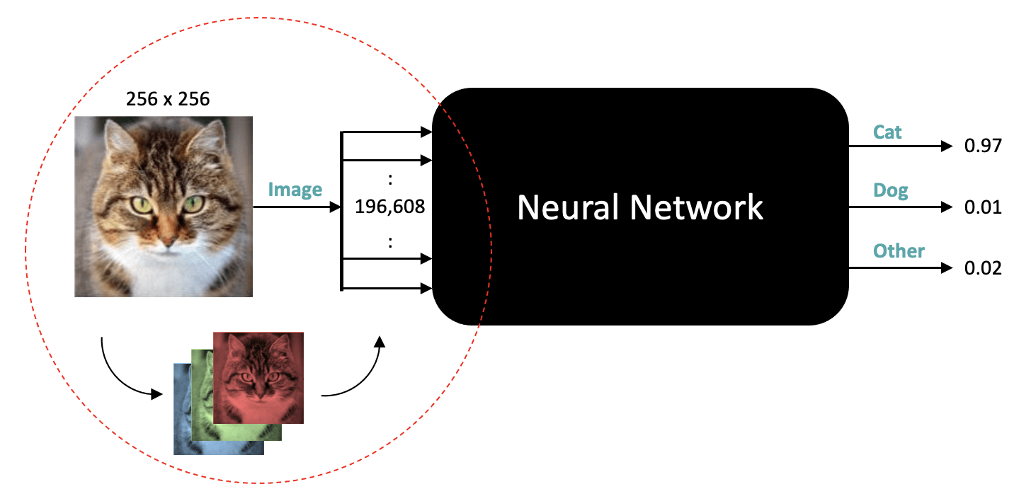
We’re going to start by treating a neural network as a black box; you have no idea what’s inside, but as you can see in this example, we have an input image of any size, format, or color and the output from the network are three numbers between 0 and 1 where each output corresponds to the probability that the input image is either a “Cat”, a “Dog” or another category which we simply call “Other.”
Understanding the Output of Neural Networks
We often refer to these categories as Labels or Class labels. This particular problem is called image classification, in which the input is an image, and the output is a numeric value for each of the three possible classes. And to be clear, the outputs from the network are three numeric values (not the labels themselves).
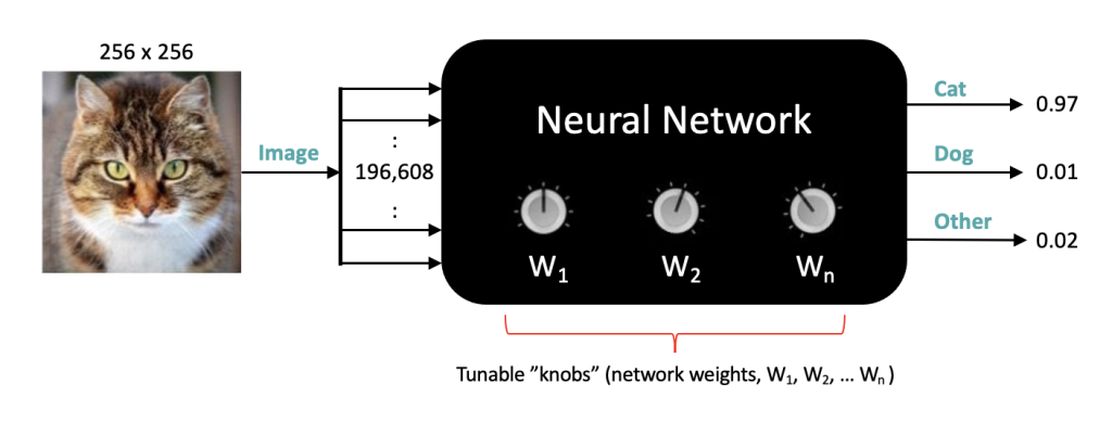
In this example, the network produces 0.97 for the first output, 0.01 for the 2nd, and 0.02 for the 3rd. Notice that the three outputs sum to one since they represent probabilities. Since the first output has the highest probability, we say the network predicted the input image to be a Cat.
More generally, the label assigned to the input image is computed by selecting the label associated with the maximum probability from the three outputs. So if the outputs were .51, .48, and .01, respectively, we would still assign the predicted label as a Cat since .51 still represents the highest probability from all three categories. In this case, the network is less confident about the prediction.
A Perfect neural network would output (1,0,0) if the input image was a cat and likewise (0,1,0) if the input image was a dog, and finally (0,0,1) if the image was something other than a cat or a dog. In reality, even well-trained networks do not give such perfect results. In practice, neural networks that perform image classification might have hundreds of possible categories (not just three, as shown here), but the process for assigning the class labels is the same. Keep in mind that neural networks can be used for many other problem types, but image classification is a very common application and well-suited as an entry-level example.


Understanding the Input of Neural Networks
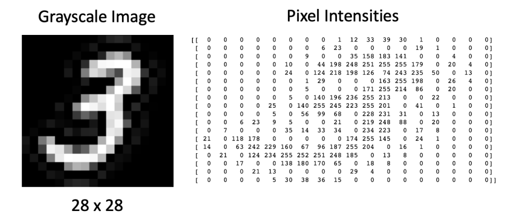
Let’s now take a look at the input to the neural network and consider how we might represent this information as numeric values. As you may already know, grayscale images are represented as an array of pixel values where each pixel value represents an intensity from pure black to pure white.
Color images are very similar, except they have three components for each pixel representing the color intensity for red, green, and blue, respectively. So, in this case, a 256 x 256 color image is represented by 196,608 numbers. With this in mind, let’s update our figure to more clearly reflect what’s happening under the hood.
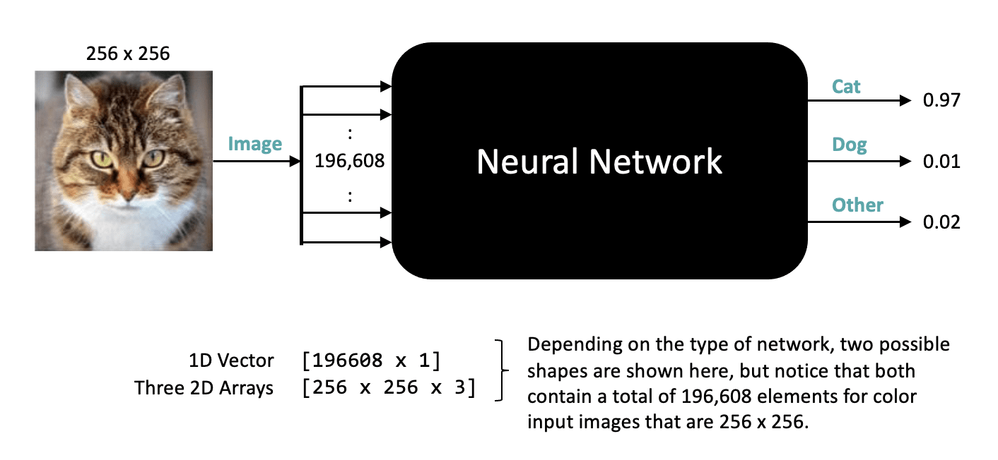
Here we are showing that the neural network expects an input that has a total of nearly 200,000 numbers, but we haven’t yet specified a shape for that data. Depending on the type of Network, the data could be represented as a 1D vector or something more compact like three 2D arrays where each array is 256×256. But in either case, a particular network design will expect a fixed size and shape for the data.
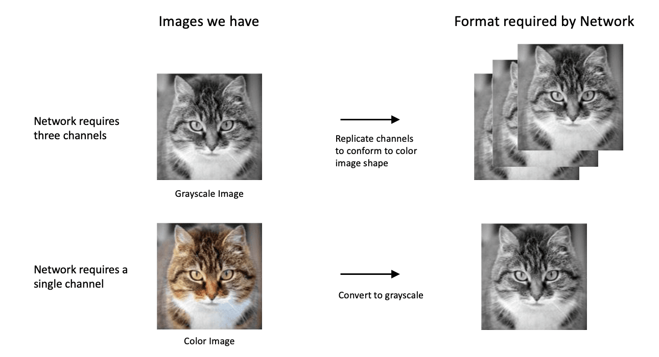
One thing that might come to mind is what happens if our input image is some other size or happens to be a grayscale image. In such cases, we can transform the image by re-sizing it or cropping it to the expected size. If the image is grayscale, we can accommodate that by replicating the single grayscale channel to make three identical channels. It’s also worth noting that some networks may only be designed to accept grayscale images, in which case color images can be converted to grayscale as a pre-processing step to create a suitable input image for the network.
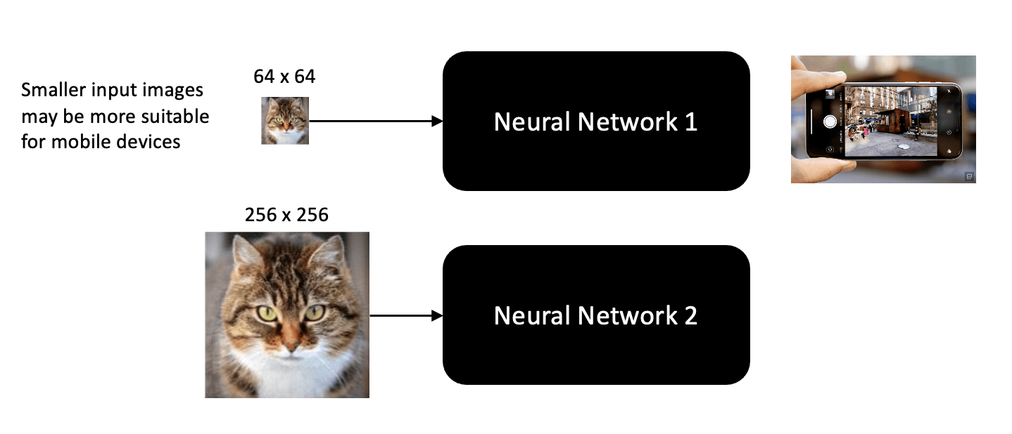
The main thing to note here is that when neural networks are designed, they are done so as to accept a certain size and shape for the input. It’s not uncommon for different image classification networks to require different size inputs depending on the application they are designed to support. For example, networks that are designed for mobile devices typically require small input images due to the limited resources that are associated with mobile devices. But that’s ok, because all we need to do is pre-process our images to conform to the size and shape required by any particular network.
What does it mean to train a Neural Network?
Let’s now talk a little bit about what it means to train a neural Network. The main thing to understand about neural networks is that they contain many tunable parameters, which you can think of as knob settings on the black box (in technical jargon, these settings are referred to as weights). If you had such a black box but didn’t know the right knob settings, it would basically be useless, but the good news is that you can find the right settings by training the neural network in a methodical manner.
The training process is analogous to how young children learn about the world around them. In everyday life, children absorb a massive amount of visual information, and through trial and error, with the help of their parents, they learn to recognize objects in the world. Training neural networks to perform image classification is very similar. It typically requires a significant amount of data and takes many iterations to determine the optimal settings for the neural network weights.
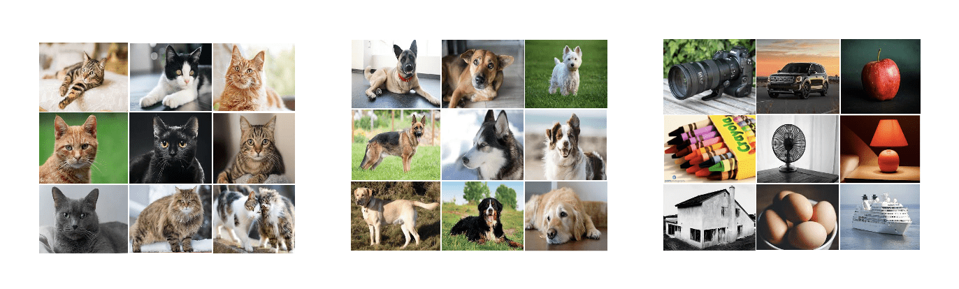
When you train a neural network, you need to show it several thousand examples of the various classes that you want it to learn, for example, images of cats, images of dogs, and images of other types of objects. This kind of training is called supervised learning because you’re providing the neural network with an image of a class and explicitly telling it that it’s an image from that class.
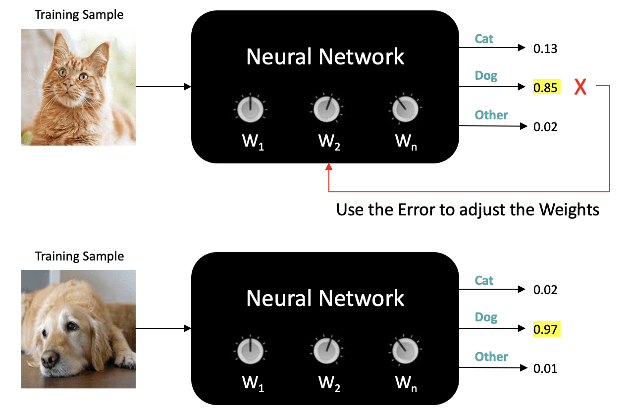
If the network makes an incorrect prediction, we compute an error associated with the incorrect prediction, and that error is used to adjust the weights in the network so that the accuracy of subsequent predictions is improved.
In the next post, we’ll delve a little deeper into how neural networks are trained, which includes how labeled training data is modeled, how loss functions are used, and the technique used to update neural network weights called gradient descent.


100K+ Learners
Join Free OpenCV Bootcamp3 Hours of Learning