

In this post, we cover the essential elements required for training Neural Networks for an image classification problem. We will still treat the internal network architecture as a black box so that we can focus on other fundamental components and concepts that are required to train neural networks.
- Introduction
- Labeled Training Data and One-Hot Encoding
- The Loss Function
- Gradient Descent (Optimization)
- Weight Update Sample Calculation
- The Complete Training Loop
- Training Plots
- Performing Inference using a Trained Model
- Conclusion
Introduction
In the previous post, we covered a high-level view of neural networks, which focused mainly on the inputs and the outputs and how the results are interpreted for an image classification problem. We also learned that neural networks contain weights that must be tuned appropriately through a training process. In this post, we will delve deeper into how neural networks are trained without getting into the details of a particular network architecture. This will allow us to discuss the training process at a conceptual level covering the following topics.
- How labeled training data is modeled.
- How a loss function is used to quantify the error between the input and the predicted output.
- How gradient descent is used to update the weights in the network.
Labeled Training Data and One-Hot Encoding
Let’s take a closer look at how labeled training data is represented for an image classification task. Labeled training data consists of images and their corresponding ground truth (categorical) labels. If a network is designed to classify objects from three classes (e.g., Cats, Dogs, Other), we will need training samples from all three classes. Typically thousands of samples from each class are required.
Datasets that contain categorical labels may represent the labels internally as strings (“Cat”, “Dog”, “Other”) or as integers (0,1,2). However, prior to processing the dataset through a neural network, the labels must have a numerical representation. When the dataset contains integer labels (e.g., 0, 1, 2) to represent the classes, a class label file is provided that defines the mapping from class names to their integer representations in the dataset. This allows the integers to be mapped back to class names when needed. As a concrete example, consider class mapping shown below.
Label    Description
  0          Cat
  1          Dog
  2          Other
This type of label encoding is called Integer Encoding because unique integers are used to encode the class labels. However, when the class labels have no relationship to one another, it is recommended that One-Hot Encoding be used instead. One-Hot encoding is a technique that represents categorical labels as binary vectors (containing only zeros and ones). In this example, we have three different classes (Cat, Dog, and Other), so we can represent each of the classes numerically with a vector of length three where one of the entries is a one, and the others are all zeros.
Cat   Dog  Other
 1     0     0
 0     1     0
 0     0     1
The particular order is arbitrary, but it needs to be consistent throughout the dataset.
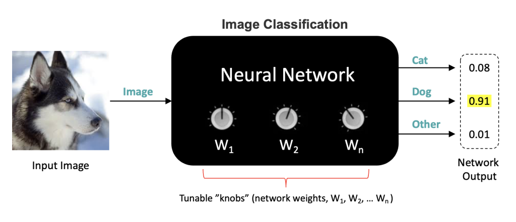
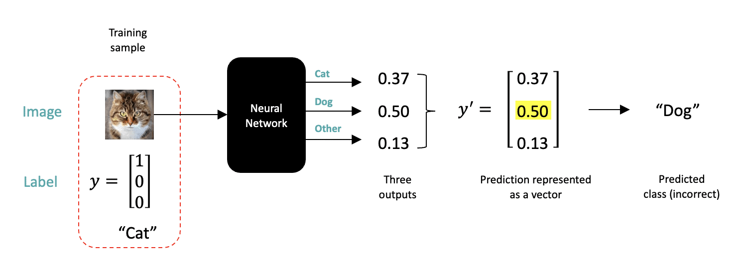
Let’s first consider a single training sample, as shown in the figure below, which consists of the input image and the class label for that image. For every input training sample, the network will produce a prediction consisting of three numbers representing the probability that the input image corresponds to a given class. The output with the highest probability determines the predicted label. In this case, the network (incorrectly) predicts the input image is a “Dog” because the second output from the network has the highest probability. Notice that the input to the network is only the image. The class labels for each input image are used to compute a loss, as discussed in the following section.
The Loss Function
All neural networks use a loss function that quantifies the error between the predicted output and the ground truth for a given training sample. As we will see in the next section, the loss function can be used to guide the learning process (i.e., updating the network weights in a way that improves the accuracy of future predictions).
One way to quantify the error between the network output and the expected result is to compute the Sum of Squared Errors (SSE), as shown below. This is also referred to as a loss. In the example below, we compute the error for a single training sample by computing the difference between the elements of the ground truth vector and the corresponding elements of the predicted output. Each term is then squared, and the total sum of all three represents the total error, which in this case, is 0.6638.

When neural networks are trained in practice, many images are used to compute a loss before the network weights are updated. Therefore, the next equation is often used to compute the Mean Squared Error (MSE) for a number of training images. The MSE is just the mean of the SSE for all the images that were used. The number of images used to update the weights is referred to as the batch size (a batch size of 32 is typically a good default). The processing of a batch of images is referred to as an “iteration.”


Gradient Descent (Optimization)
Now that we are familiar with the concept of a loss function, we are ready to introduce the optimization process used to update the weights in a neural network. Fortunately, there is a principled way to tune the weights of a neural network called gradient descent. For simplicity, we’re going to illustrate the concept with just a single tunable parameter called  , and we’re going to assume the loss function is convex and therefore shaped like a bowl, as shown in the figure.
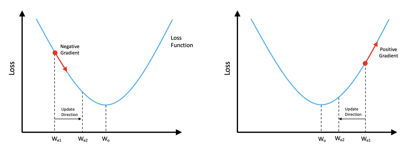
The value of the loss function is shown on the vertical axis, and the value of our single trainable weight is shown on the horizontal axis. Let’s assume the current estimate of the weight is  .
.
Referring to the plot on the left, If we compute the slope of the loss function at the point corresponding to the current weight estimate , we can see that the slope (gradient) is negative. In this situation, we would need to increase the weight to get closer to the optimum value indicated by  . So we would need to move in a direction opposite from the sign of the gradient.
On the other hand, if our current weight estimate,  (as shown in the plot to the right), the gradient would be positive, and we would need to reduce the value of the current weight to get closer to the optimum value of . Notice that in both cases, we still need to move in a direction opposite from the sign of the gradient.
Before we continue, let’s clarify one point in case you’re wondering. Notice that, in both figures, the arrow that we’ve drawn to represent the gradient (slope) is pointing to the right. In one case, the arrow is pointing down and to the right, and in the other, the arrow is, pointing up and to the right. But don’t be confused by the fact that both arrows are pointing toward the right, what’s important is the sign of the gradient,
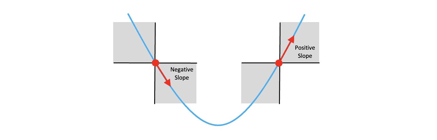
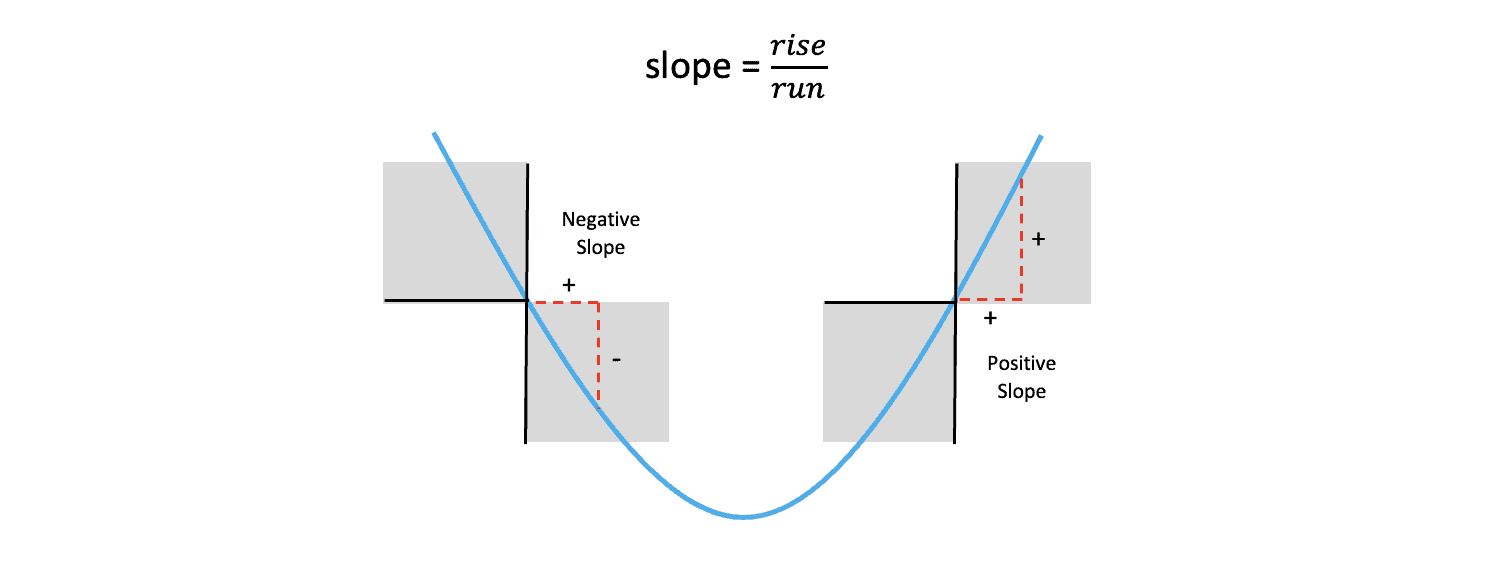
Remember that the slope of a line is defined as the rise over the run and that when the weight is to the left of the optimum value, the slope of the function is negative, and when the weight is to the right of the optimum value, the slope of the function is positive. So it’s the sign of the gradient that’s important.
In both cases described above, we need to adjust the weight in the direction that is opposite from the sign of the gradient. With these concepts in mind, we can show that the following equation can be used to update the weight in the proper direction regardless of the current value of the weight relative to the optimal value.
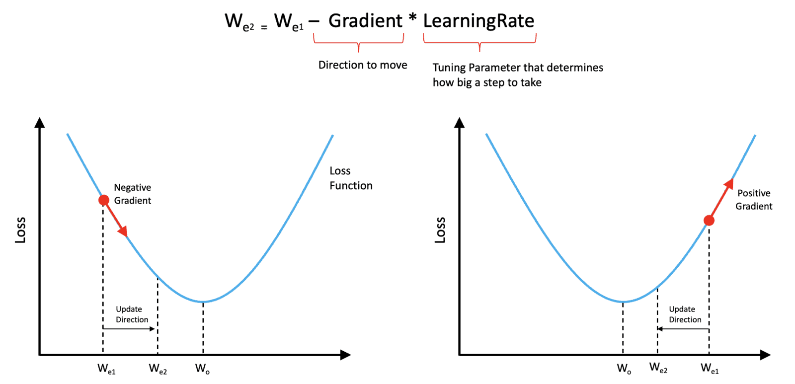
The best way to think about this is that the sign of the gradient determines the direction we need to move in. But the amount that we need to move needs to be tempered with a parameter called the learning rate, which is often a small number much less than 1. The learning rate is something that we need to specify prior to training and is not something that is learned by the network. Parameters like this are often called hyperparameters to distinguish them from trainable parameters (such as the network weights).
In practice, the loss function has many dimensions and is not typically convex but has many peaks and valleys. In the general case, the slope of the loss function is called the gradient and is a function of all the weights in the network. But the approach used to update the weights is conceptually the same as described here.
Weight Update Sample Calculation
To make this a little more concrete, let’s do a sample calculation for updating the weight. Here let’s assume that the current weight is  , which has a value of
 0.38. We will also assume that we have a learning rate of .01 and that the slope of the loss function at the point is equal to -.55. Using the update equation above, we can easily compute a new estimate for the weight which we will refer to as  . This calculation was simplified because we’re working in just a single dimension, which is easily extended to multiple dimensions.
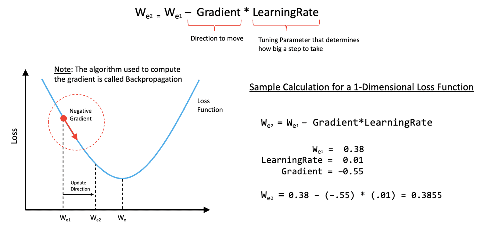
One thing we haven’t talked about yet is how you actually compute the gradient of the loss function with respect to the weights in the network. Fortunately, this is handled by an algorithm called backpropagation, which is built into deep learning frameworks, such as TensorFlow, Keras, and PyTorch, so it’s not something you need to implement yourself.
The Complete Training Loop
Now that we’ve covered all the essential elements associated with training a neural network, we can summarize the process in the following diagram.
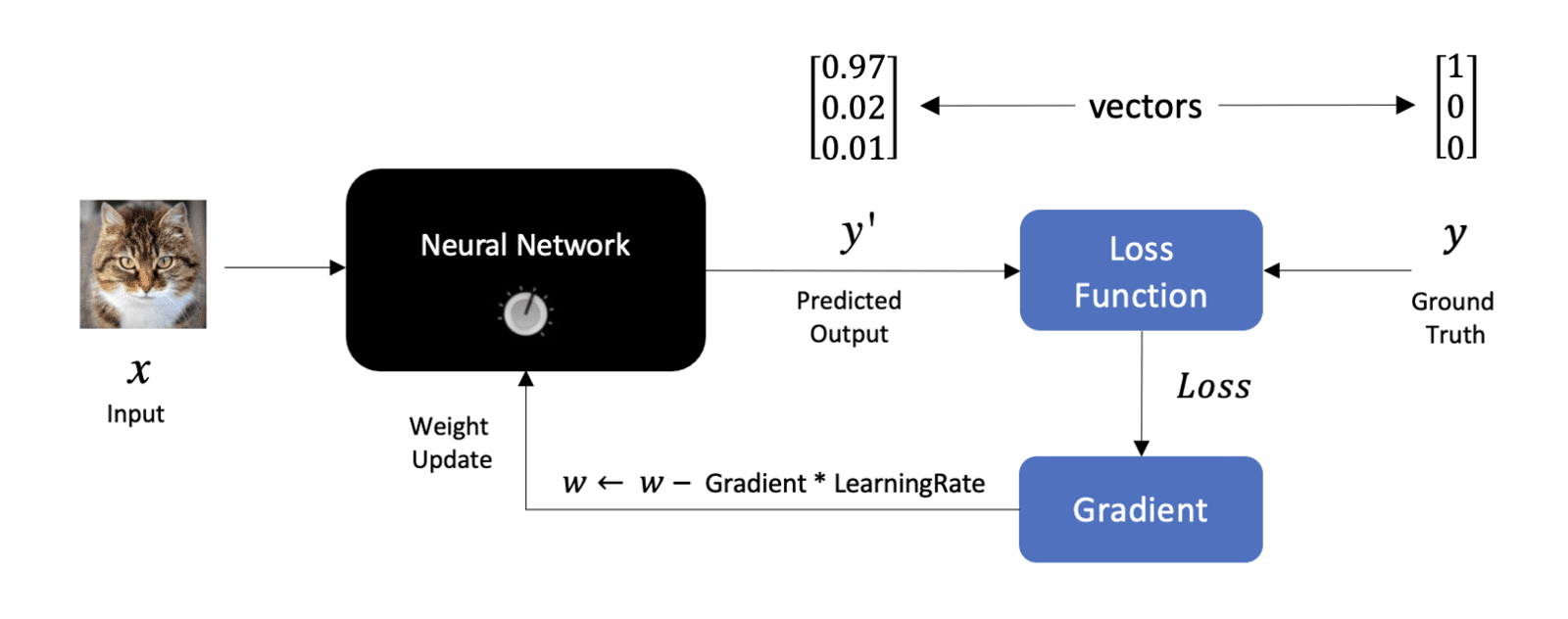
Here, we have an input image on the left and the output from the network on the right, which we refer to as  . We use the ground truth label,
  , along with the predicted output from the Network to compute a loss. Notice that we don’t specifically show multiple outputs from the network, but it’s should be understood that both and are vectors whose length is equal to the number of classes that the network is being trained for.
After we compute the loss, we can compute the gradient of the loss with respect to the weights, which can then be used to update the weights in the Network. This is an important diagram that summarizes at a high level the process of training a neural network.
Training Plots
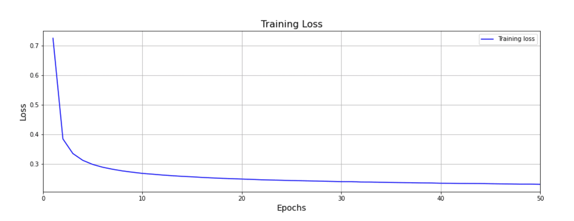
Now that we have an idea as to how we can update the weights in a network, it’s worth emphasizing that training a neural network is an iterative process that typically requires passing the entire training set through the Network multiple times.
Each time the entire training dataset is passed through the network, we refer to that as a training epoch. Training neural networks often require many training epochs until the point where the loss stops decreasing with additional training. As you can see in the first plot below, the rate at which the loss decreases tapers off as training progresses, indicating that the model is approaching its capacity to learn.
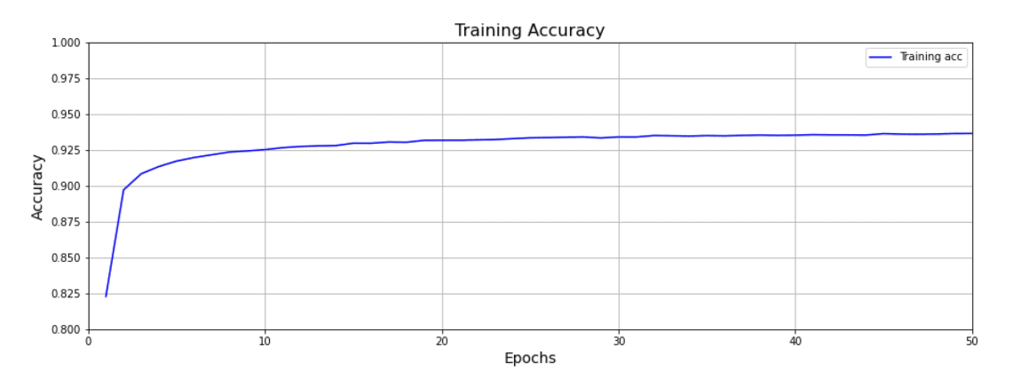
It’s also very common to plot training accuracy, and as you might expect, as the loss decreases, the accuracy tends to increase as shown in the second plot.
There are many important details associated with training neural networks that we have not covered in this initial post, but as we progress through this series, we’ll continue to introduce more advanced concepts on this topic.
Note: One important topic that we have not yet covered is data splitting. This involves the concept of a validation dataset used to evaluate the quality of the trained model during the training process. This is an important and fundamental topic that will be covered in a subsequent post.
Performing Inference using a Trained Model
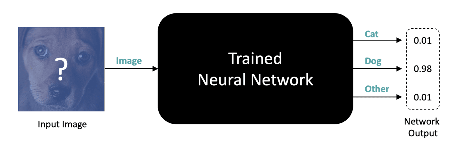
Now that we’ve covered the process for how to train a neural network, it’s worth talking a little bit about what we’re going to do with it. Once we have a trained Network, we can supply it with images of unknown content and use the network to make a prediction as to what class the image belongs to. This is reflected in the diagram below, and notice that at this point, we do not require any labeled data. All we need are images with unknown content that we wish to classify. Making predictions on unknown data is often referred to as using the network to perform inference.
Conclusion
Let’s summarize the key points associated with training neural networks.
- Labeled training data is required to train a neural network for supervised learning tasks such as image classification.
- One-Hot label encoding is recommended for categorical data in most cases.
- Training a neural network requires a loss function which is used to quantify the error between the network output and the expected output.
- The Gradient of the loss function is computed using an algorithm called Backpropagation which is built into Deep Learning frameworks like TensorFlow and PyTorch.
- Gradient Descent is used in an iterative manner to update the weights of the neural network.
- A subset of the training images (batch size) is used to perform a weight update. This is referred to as an iteration within a training epoch.
- A training epoch consists of processing the entire training dataset through the network. So the number of iterations in a training epoch equals the number of training images divided by the batch size.
- Each training epoch represents a full pass of the training progresses until the loss function stabilizes. Caution: In practice, we don’t rely solely on the training loss to assess the quality of the trained model. Validation loss is also required, which we will cover in a subsequent post.
100K+ Learners
Join Free OpenCV Bootcamp3 Hours of Learning