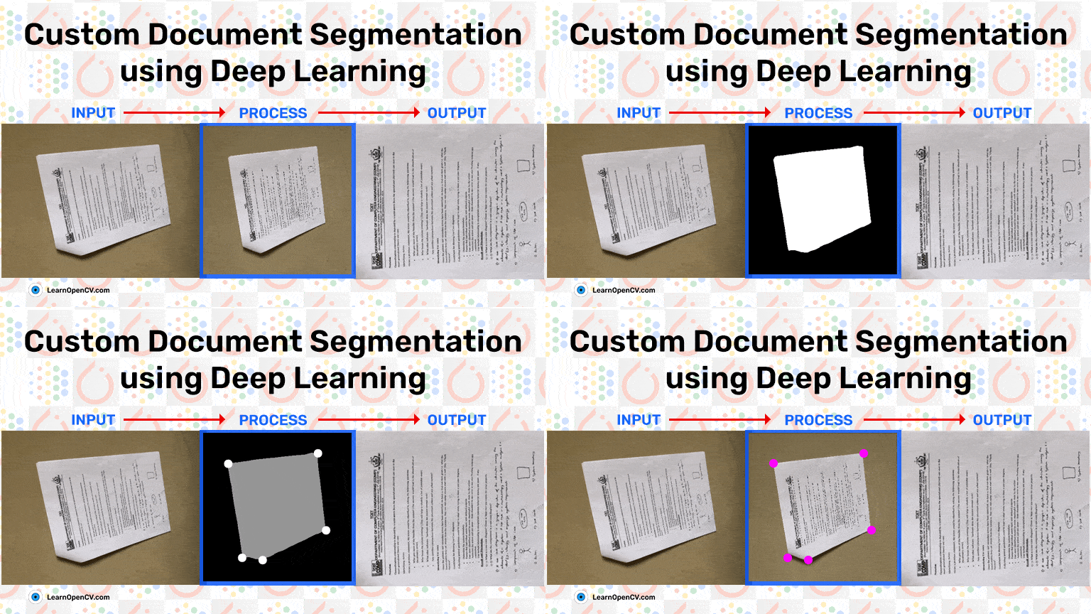
Document Scanning is a background segmentation problem that can be solved using various methods. It is one of the extensively used applications of computer vision. In this article, we are considering Document Scanning as a deep learning-based semantic segmentation problem. This article will show how to load and train DeepLabv3 in PyTorch for Document Segmentation on a synthetic dataset. We have also deployed the app on streamlit that you can use freely.
Document Segmentation Using Deep Learning in PyTorch [TL;DR]
Previously, we explored classical computer vision techniques in an effort to automate the pipeline. Check out the post “Automatic Document Scanner using OpenCV”, where we created a Document Scanner using only OpenCV. However, as documented, imperfections were observed in some cases. The reason for failure was our biased assumption regarding the structure and placement of the documents and background variations.
In this article, we will train a semantic segmentation model on a custom dataset in PyTorch.
The steps for creating a document segmentation model are as follows.
- Collect dataset and pre-process to increase the robustness with strong augmentation.
- Build a custom dataset class generator in PyTorch to load and pre-process image mask pairs.
- Select and load a suitable deep-learning architecture.
- Choose appropriate loss function and evaluation metrics to train the model.
- Image Segmentation Prerequisites
- Why use a deep learning-based solution for Document Segmentation?
- Workflow for Training a Custom Semantic Segmentation Model
- Preparing Synthetic Dataset for Robust Document Segmentation
- A Custom Dataset Class for Loading Documents and Masks
- Loading Pre-trained DeeplabV3 Semantic Segmentation Models
- Selecting Loss and Metric Functions IoU and Dice
- Custom Training Image Segmentation Model
- Inference and Comparison of Results
- Summary: Document Segmentation
- References
1. Image Segmentation Prerequisites
This post assumes that you are familiar with the basic concepts of Image Segmentation, Semantic segmentation, and the workings of Pytorch. If not, we’ve got you covered.
- You can refer to our article on Image segmentation, where we have covered the basics and types of segmentation in detail.
- We have a series of excellent posts for getting started with PyTorch, which you can use to familiarize yourself with the fundamentals of PyTorch.
2. Why use a deep learning-based solution for Document Segmentation?
Robustness. As observed in the previous post of the series, for a document scanner to perform effectively across multiple scenarios is a challenging task. To be robust, the algorithm used must be free of biased assumptions. Our approach uses a deep learning-based image segmentation model trained on different scenarios to create a robust segmentation model.
3. Workflow For Training A Custom Semantic Segmentation Model
The steps for creating a robust custom document segmentation model are as follows:
- As with any project, after defining the problem statement, the next crucial step is to figure out the dataset collection procedure, i.e. how do we go about collecting the dataset for the task?
- The aim is to create a document segmentation model that works competently in multiple scenarios. To do so, we will generate a Synthetic dataset using background and document images collected from various sources.
- After creating the synthetic dataset, we move on to PyTorch to create a custom Dataset class generator. It will be responsible for loading and preprocessing the image-mask pairs.
- Next, we’ll load the deep learning model for the task. There are many pre-trained models readily available in PyTorch. Here, we are using DeeplabV3 with MobilenetV3-Large backbone.
- Before we start training the model, the final component is selecting the appropriate loss functions and evaluation metrics. We’ll briefly discuss the two most common concepts, Intersection over Union and Dice Coefficient, used for segmentation problems and select the one most useful for our task.
We’ll train our custom semantic segmentation model and compare the results with the document extraction approach used in the previous post and on the DocUNet dataset.
4. Preparing Synthetic Dataset For Robust Document Segmentation
A general breakdown of time spent in any machine learning or deep learning project is estimated to be 80% for the dataset collection, preparation and analysis. Only 20% of the remaining time goes into actual training and improvements.
We aim to create a robust document segmentation model. To do so, we need a dataset containing various documents in multiple backgrounds captured in different orientations. As you can imagine, collecting such a dataset is very time-consuming (typical for any project), so we take the other route.
Here, we generate a synthetic dataset that closely resembles the different problems (such as motion blur, camera noise, etc.) associated when capturing real-world images. This procedure helps us overcome some of the shortcomings of a manually created dataset and removes the hassle of capturing pictures and annotation.
4.1 Gathering and Pre-Processing of Document and Background Image
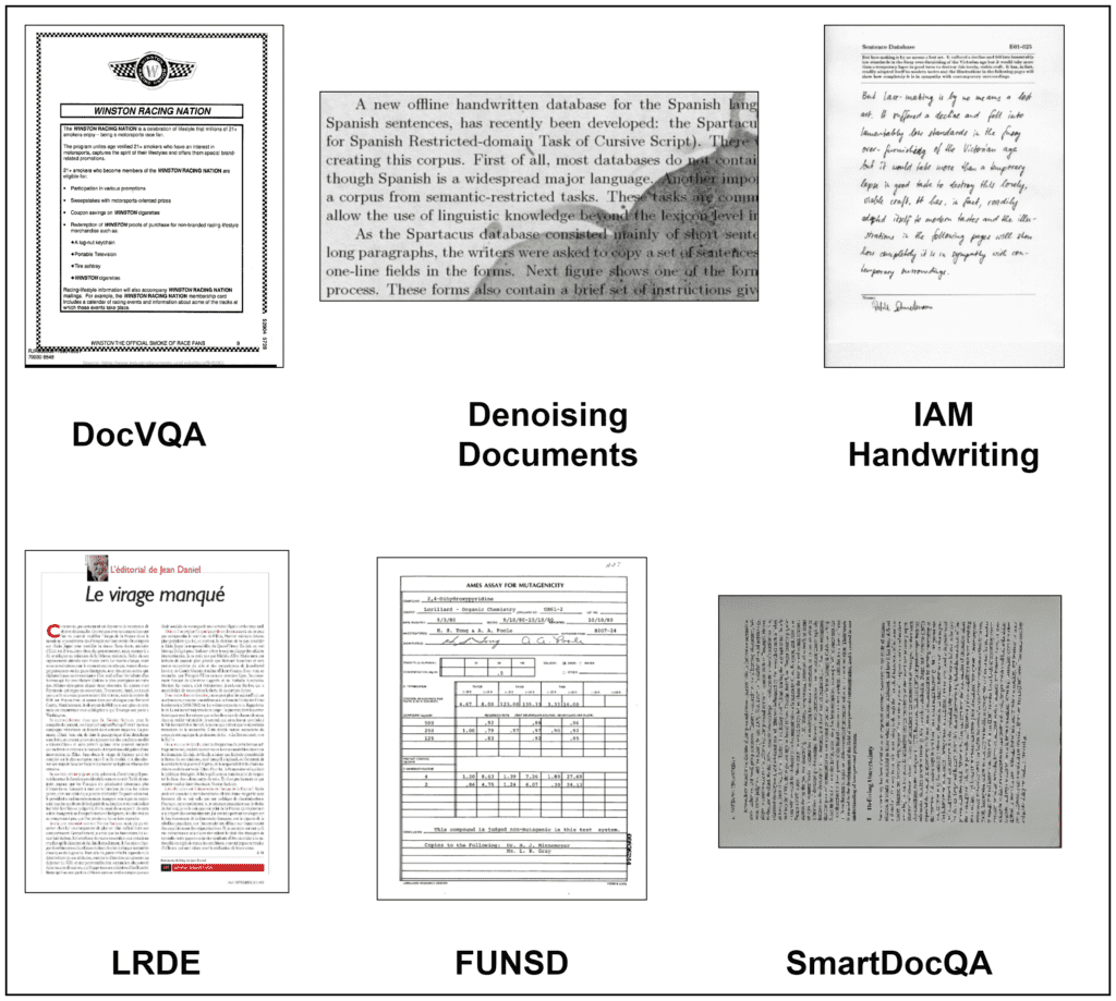
To generate a synthetic dataset, we need the following sets of images.
- Images of different types of Documents.
- A wide variety of Background images.
| Datasets | Total Images Present | Number of Images taken (randomly) |
| 1. Val and Test set from DocVQA | 2573 | 700 |
| 2. IAM Handwriting Database | 522 | 100 |
| 3. Denoising Dirty Documents | 360 | 125 |
| 4. FUNSD | 199 | 199 |
| 5. LRDE Document Dataset | 125 | 125 |
| 6. SmartDoc QA | 4260 | 85 |
| TOTAL DOCUMENTS | 1343 |
Table 1: Details regarding Document image sources and the number of images used.
Following are the steps involved in pre-processing of images.
- Images in the above sources vary a lot in terms of dimensions. As a result, all documents were resized (aspect ratio maintained) with the maximum dimension size set to 640. This is done to induce some structure in the documents and decrease processing time.
- As all images are cropped documents, the mask for each document is generated by creating an array of the same shape filled with the value 255.
- SmartDoc QA contains 4260 raw images, of which 85 documents were manually annotated and extracted.
Background images: One of the goals for generating a synthetic set is to simulate the situations where documents are placed in different backgrounds. We can use Google image search results to create a background image dataset. The dataset was created by downloading images resulting from queries such as “table images top view,” “laminate sheet close up image,” “Wooden table close up,” etc. The queries used were such that they resulted in images with different textures and colors.
To ease the download process, we used this fork of the Google Images Download repository. All images were either downloaded or converted to JPG format. After filtering out the duplicate images, we were left with 1055 background images.
4.2 Procedure for Generating Synthetic Dataset for Document Segmentation
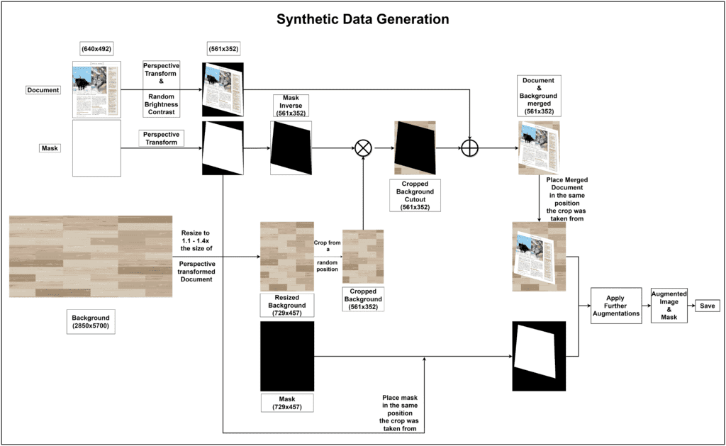
The above diagram shows the flow for generating one image and mask pair. The main goal of synthetic data generation is to have documents placed across various backgrounds and positions. So, each document-mask pair is subjected to RandomPerspective (with RandomBrightnessContrast (50% probability) for documents) transformation 6 times, with a 70% probability that the transformation will be applied.
For the 6 transformed documents and mask images, 6 background images from the entire set are randomly selected. The transformed document and the chosen background images are then merged together. Each merged output pair (image and mask) is subjected to further augmentations to replicate the real-world scenario as closely as possible.
The augmentation set consists of the following modifications.
- Horizontal and Vertical Flipping
- RandomRotation
- Colour Jitter
- Channel Shuffle
- Random Brightness and Contrast
- One of: Image Compression, ISO Noise, Motion Blur
- One of: Random Shadow, Sun-Flare, RGB shift
- One of Optical Distortion, Grid Distortion or Elastic Transformation
All except Perspective transformation are applied using the Albumentations library.
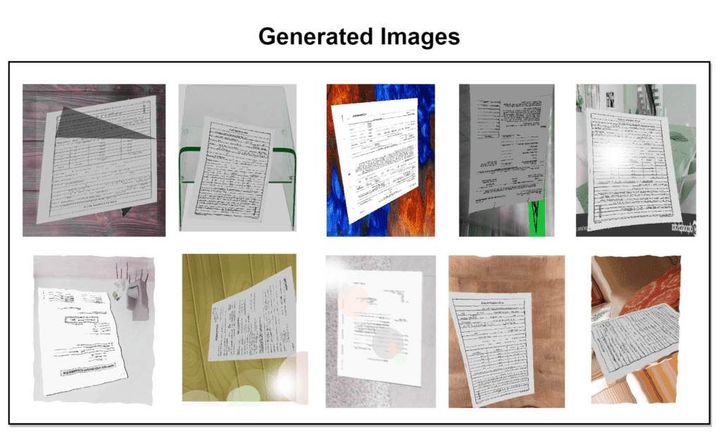
A total of 8058 image-mask pairs were generated, out of which 6715 were selected for the training set, and the remaining 1343 made up the validation set.
5. A Custom Dataset Class for Loading Documents and Masks
A custom Dataset class is created to load and convert an image and mask pair into the appropriate format. All steps except the preprocess transformations for images are similar for the training and validation set. For the train set, an additional augmentation, “RandomGrayscale”, is applied to the images with a probability of 40%.
The additional augmentation is used to make training a little more challenging. This forces the model to focus more and better learn the difference between (any type of) document and background. The decision was taken after observing the results from multiple experiments. When training a model for only grayscaled or only RGB images, both perform well but fail in places where the other seems to work well.
- The mask for each image consists of 2 channels – one for the background and the other for the document.
- All images and masks returned are first rescaled to the range [0. , 1.]. Images are further normalized according to ImageNet mean and std. dev. statistics.
The following block contains the code to prepare the document segmentation dataset.
import torchvision.transforms as torchvision_T

def train_transforms(mean=(0.4611, 0.4359, 0.3905),
                      std=(0.2193, 0.2150, 0.2109)):
    transforms = torchvision_T.Compose([
        torchvision_T.ToTensor(),
        torchvision_T.RandomGrayscale(p=0.4),
        torchvision_T.Normalize(mean, std),
    ])
    return transforms


def common_transforms(mean=(0.4611, 0.4359, 0.3905),
                       std=(0.2193, 0.2150, 0.2109)):
    transforms = torchvision_T.Compose([
        torchvision_T.ToTensor(),
        torchvision_T.Normalize(mean, std),
    ])
    return transforms


class SegDataset(Dataset):
    def __init__(self, *,
                 img_paths,
                 mask_paths,
                 image_size=(384, 384),
                 data_type="train"
    ):

        self.data_type  = data_type
        self.img_paths  = img_paths
        self.mask_paths = mask_paths
        self.image_size = image_size

        if self.data_type == "train":
            self.transforms = train_transforms()
        else:
            self.transforms = common_transforms()

    def read_file(self, path):
        file = cv2.imread(path)[:, :, ::-1]
        file = cv2.resize(file, self.image_size,
                          interpolation=cv2.INTER_NEAREST)
        return file
    def __len__(self):
        return len(self.img_paths)

    def __getitem__(self, index):
        image_path = self.img_paths[index]
        image = self.read_file(image_path)
        image = self.transforms(image)

        mask_path = self.mask_paths[index]
        gt_mask = self.read_file(mask_path).astype(np.int32)

        _mask = np.zeros((*self.image_size, 2), dtype=np.float32)

        # BACKGROUND
        _mask[:, :, 0] = np.where(gt_mask[:, :, 0] == 0,   1.0, 0.0)

  # DOCUMENT
        _mask[:, :, 1] = np.where(gt_mask[:, :, 0] == 255, 1.0, 0.0)

        mask = torch.from_numpy(_mask).permute(2, 0, 1)
        return image, mask
The dataset object for the training and validation set is initialized with appropriate arguments and then wrapped around a DataLoader object.

6. Loading Pre-Trained DeeplabV3 Semantic Segmentation Models
The PyTorch framework provides three pre-trained variants of the model. The main difference between them is the backbone model. For document segmentation, we chose the model with the MobileNetV3-Large backbone. The model is smaller than the other variants but has a good mIoU score and high inference speed. It has over 11M+ parameters and was trained on a subset of COCO, using only the 20 categories in the Pascal VOC dataset.
DeepLabv3 is considered one of the milestones of deep learning-based semantic segmentation models. Released in late ’17, the architecture quickly gained popularity because of its incredible speed, accuracy, and simplicity. For these reasons, we have written an in-depth, one-stop guide to DeepLabv3 architecture for you, where we explore the various components of both DeepLabv3 and DeepLabv3+ in detail.
We will fine-tune all the model layers as our target class differs significantly from the classes used for training the model.
from torchvision.models.segmentation import deeplabv3_mobilenet_v3_large
from torchvision.models.segmentation import deeplabv3_resnet50, deeplabv3_resnet101

def prepare_model(backbone_model="mbv3", num_classes=2):
    weights = 'DEFAULT'    # Initialize model with pre-trained weights.
    if backbone_model == "mbv3":
        model = deeplabv3_mobilenet_v3_large(weights=weights)
    elif backbone_model == "r50":
        model = deeplabv3_resnet50(weights=weights)
    elif backbone_model == "r101":
        model = deeplabv3_resnet101(weights=weights)
    else:
        raise ValueError("Wrong backbone model passed. Must be one of 'mbv3', 'r50' and 'r101' ")

    # Update the number of output channels for the output layer.
    # This will remove the pre-trained weights for the last layer.
    model.classifier[4]         = nn.LazyConv2d(num_classes, 1)
    model.aux_classifier[4] = nn.LazyConv2d(num_classes, 1)

    return model
# Dummy Initialization.
model = prepare_model(num_classes=2)
model.train()
# In train mode, batch size needs to be at least 2.
out = model(torch.randn((2, 3, 384, 384)))
print(out['out'].shape) # torch.Size([2, 2, 384, 384])
7. Selecting Loss and Metric Functions IoU and Dice
So far, we have worked through the details of the Dataset class and a function to initialize the model. Next, we need to select the appropriate loss function and evaluation metric suitable for the task.
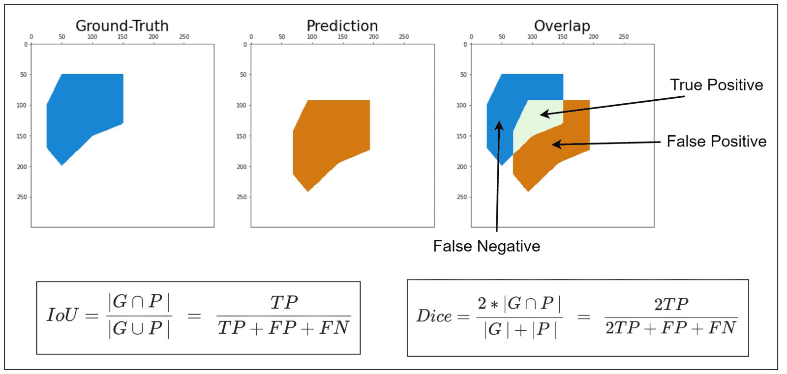
Two methods are widely preferred for segmentation problems. Both can be used as a loss function or an evaluation metric. They are:
- Intersection over Union (IoU) is a metric often used to assess the model’s accuracy in segmentation problems. It provides a more intuitive basis for accuracy that is not biased by the (unbalanced) percentage of pixels from any particular class.
- Dice Coefficient (otherwise known as the F1-Score) is another metric used in the segmentation context and is very similar to IoU. Simply put, the metric is twice the overlap area divided by the total number of pixels in both ground truth and prediction.
Both metrics range from 0 to 1 and are positively correlated.
“The point of difference occurs when penalizing the wrong predictions. IoU penalizes FP and FN predictions twice more than Dice.”
With some minor differences (w.r.t. post-processing of model predictions), we can use both methods as loss and metric functions (loss = 1 – metric). The core computation remains the same. For this reason, a joint function is defined that returns the metric value.
7.1 Implementing Loss Function and Evaluation Metric
The custom document segmentation model is trained using a Combo Loss of IoU and Binary Cross-entropy, and we use naive IoU as the evaluation metric.
def intermediate_metric_calculation(predictions, targets, use_dice=False, smooth=1e-6, dims=(2,3)):
    # dims corresponding to image height and width: [B, C, H, W].
    # Intersection: |G ∩ P|. Shape: (batch_size, num_classes)
    intersection = (predictions * targets).sum(dim=dims) + smooth

    # Summation: |G| + |P|. Shape: (batch_size, num_classes).
    summation = (predictions.sum(dim=dims) + targets.sum(dim=dims)) + smooth

    if use_dice:
        # Dice Shape: (batch_size, num_classes)
        metric = (2.0 * intersection) / summation
    else:
        # Union. Shape: (batch_size, num_classes)
        union = summation - intersection

        # IoU Shape: (batch_size, num_classes)
        metric = intersection /  union

    # Compute the mean over the remaining axes (batch and classes).
    # Shape: Scalar
    total = metric.mean()
    return total
The main code for the Loss Class:
# Normalize model predictions.
predictions = torch.sigmoid(predictions)

# Calculate pixel-wise loss for both channels. Shape: Scalar
pixel_loss = F.binary_cross_entropy(predictions, targets, reduction="mean")

mask_loss = 1 - intermediate_metric_calculation(predictions,   targets,
                                                			use_dice=self.use_dice,  smooth=self.smooth)
# Return total_loss
total_loss = mask_loss + pixel_loss
Similarly, for the Metric Class:
# Convert unnormalized predictions into one-hot encoded across channels.
# Shape: (B, #C, H, W)
predictions = convert_2_onehot(predictions, num_classes=self.num_classes)
# Return metric
metric = intermediate_metric_calculation(predictions,  targets,
					use_dice=self.use_dice, smooth=self.smooth)
The convert_2_onehot function is a separate helper function for converting model predictions across channels into one-hot values.
8. Custom Training Document Segmentation Model
Now that we have defined all the components required, we are ready to train our custom semantic segmentation model for document segmentation. The hyperparameters and results for the final training were as follows.
| 1. Backbone Model | MobileNetV3-Large |
| 2. Image Shape | (384 x 384 x 3) |
| 3. Mask Shape | (384 x 384 x 2) |
| 4. Number of output channels | 2 (0 – background, 1 – document) |
| 5. Number of Epochs Trained | 50 |
| 6. Batch Size | 64 |
| 7. Optimizer | Adam |
| 8. Learning Rate | 0.0001 (Constant) |
| 9. Loss Function/s | Binary Cross entropy + Intersection over union (BCE + IoU) |
| 10. Evaluation Metric | Intersection over Union (IoU) |
| 11. Best Loss Values | Training – 0.027 |
| Validation – 0.076 | |
| 12. Best Metric Scores | Training – 0.989 |
| Validation – 0.976 |
Table 2: Training hyperparameters and final scores
We also trained Deeplabv3 with the Resnet-50 backbone using the same hyperparameters mentioned in the table above but trained for 25 epochs. Empirically, the difference was only about +0.07. Still, we preferred the lightweight MobileNetv3-large variant due to its speed, allowing us to conduct more experiments quickly.
During experimentation, multiple combinations of different hyperparameters were tested. These include Dice + BCE loss function, single channel output, different image sizes, all grayscale images, all RGB images, with and without class weight masks, etc. The hyperparameters stated in the above table resulted in the best performance.
9. Inference and Comparison of Results
A test set of 51 images was created, which consists of 23 (including failure case) images from the previous post and 28 newly captured images.
The results are shown for the 25 images that exhibit major differences. The models perform really well, and we can clearly see the difference between the two approaches.

Fig: Document Segmentation Comparison Results
Further, models were tested on the cropped version of the DocUNet dataset.
Results:
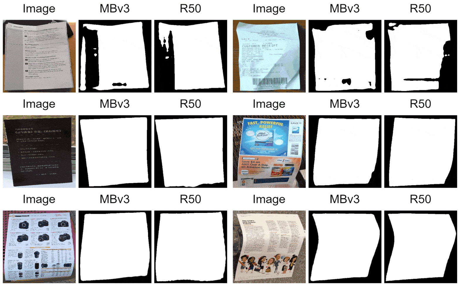
Testing on the DocUNet dataset indicates there’s still room for further improvements in the synthetic dataset generation procedure and the training process, but that’s for another time.
10. Summary
In this post, our goal was to improve our previously used document extraction approach with something that’s much more robust. To do so, we moved away from the traditional CV algorithms and created a deep learning-based custom semantic segmentation model for document segmentation. A deep learning-based approach allows us to be free of any assumptions we had to make when working with traditional CV algorithms.
This post covered generating a synthetic dataset, defining appropriate loss and metric functions for image segmentation, and training a custom DeeplabV3 model in PyTorch. The results presented in the Inference and Comparison Results section indicate that a deep learning-based approach significantly improved over the previous method. But that’s not it; as demonstrated from testing on the DocUNet dataset, there’s still room for improvement.
11. References
- Automatic Document Scanner Using Opencv
- Image Segmentation
- Rethinking Atrous Convolution for Semantic Image Segmentation
- Searching for MobileNetV3
- DocUNet: Document Image Unwarping via A Stacked U-Net








100K+ Learners
Join Free OpenCV Bootcamp3 Hours of Learning