DeepLabv3 & DeepLabv3+ The Ultimate PyTorch Guide

DeepLab models, first debuted in ICLR ‘14, are a series of deep learning architectures designed to tackle the problem of semantic segmentation. After making iterative refinements through the years, the same team of Google researchers in late ‘17 released the widely popular “DeepLabv3”. DeepLabv3, at the time, achieved state-of-the-art (SOTA) performance on the Pascal VOC 2012 test set and on-par SOTA results on the famous Cityscapes dataset and when trained with Google’s in-house JFT dataset.

DeepLabv3+, presented at ECCV ‘18, is the incremental update to DeepLabv3. It made fundamental architectural changes on top of the DeepLabv3 semantic segmentation model. 

DeepLabv3+ (2018) surpassed 🏆 DeepLabv3 (2017) model and achieved SOTA mIOU performance on both the PASCAL VOC 2012 test set (89%) and the Cityscapes dataset (82.1%).

In this article, we will explore various aspects of DeepLabv3 and will cover the following: 

1. What is DeepLabv3?
2. The problems & solutions faced in segmentation.
3. The architecture of DeepLabv3.
4. What is DeepLabv3+?
5. Architectural updates to DeepLabv3+.
6. Semantic Segmentation using PyTorch.

1. What Is DeepLabv3?
2. DeepLabv3 Solution To Problems Faced In Segmentation
3. Components Of DeepLabv3
   1. Atrous Convolution
   2. Atrous Spatial Pyramid Pooling (ASPP)
4. DeepLabv3 Architecture
   1. Atrous Convolution Arranged In A Cascade
   2. Atrous Convolution Arranged In Parallel
   3. DeepLabv3 On The Pascal VOC Test Set
5. Going From DeepLabv3 To DeepLabv3+
6. Components & Architecture Of DeepLabv3+
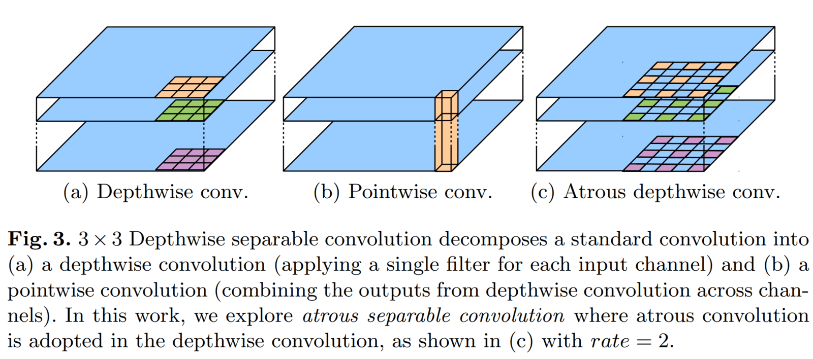
7. What Is Atrous Separable & Depthwise Separable Convolution?
8. DeepLabv3+ Paper Experiments
   1. DeepLabv3+ On The Pascal VOC Test Set
   2. DeepLabv3+ On Cityscapes Test Set
9. Semantic Segmentation Using DeepLabv3 in PyTorch
   1. Loading PyTorch DeepLabv3 Models
10. Summary

What Is DeepLabv3?

DeepLabv3 is a fully Convolutional Neural Network (CNN) model designed by a team of Google researchers to tackle the problem of semantic segmentation. DeepLabv3 is an incremental update to previous (v1 & v2) DeepLab systems and easily outperforms its predecessor.

The previous generations of DeepLab systems used “DenseCRF,” a non-trainable module, for accuracy refinement in post-processing. Since then, DeepLabv3 has completely dropped the post-processing module and is an end-to-end trainable deep learning system.

Deeplabv3 cemented its status as one of the go-to models for segmentation because of its:

1. High speed
2. Better accuracy,
3. Architectural simplicity. 
4. Generalizability to custom tasks. 

From an architectural standpoint, DeepLabv3 uses the ResNet models (trained on Imagenet) as the backbone along with the widely popular Atrous Convolution (more commonly known as “dilated convolutions”) and Atrous Spatial Pyramid Pooling (ASPP) module. 

The significant contributions of the DeepLabv3 paper are:

1. A general framework that one can use in any network.
2. The drawbacks of using a large dilation rate.
3. An improved ASPP module.

DeepLabv3 Solution To Problems Faced In Segmentation

A general approach to creating a segmentation model is to use a model trained on benchmark classification datasets such as Imagenet. As these models need to classify up to 1000 classes, the essential requirement is to be able to extract features that are general in nature. These models undergo rigorous experimentation in their development phase before being released. Due to this, pre-trained models are commonly used for several downstream tasks such as object detection, segmentation, etc.

Problems:

Due to consecutive pooling or strided convolutions for downsampling, the “feature resolution decreases as we go deeper into the network.” Downsampling blocks are widely adopted in deep convolutional neural networks (CNN) as they help reduce memory consumption while preserving the transformation invariance.

This behavior is beneficial for image classification but is troublesome for segmentation tasks, where spatial information is necessary. As we go deeper into the network, the feature maps become increasingly good at encoding “what is in the image?” but the information about “where in the image?” is lost.

The second problem is the “existence of objects at multiple scales.”  For example, the “person” class can be present in multiple resolutions in an image. As we go deeper into the networks, the receptive field increases, becoming increasingly good at detecting large objects. However, in the process, smaller size objects suffer.

The solution used in DeepLabv3:

1. To alleviate the first problem, Deeplabv3 uses “Atrous Convolution” along with some changes to the backbone’s pooling and convolutional striding components.
2. For the second problem, a modified “Atrous Spatial Pyramid Pooling” module is used for multi-scale feature extraction.

“For semantic segmentation, it has been shown that global features or contextual interactions are beneficial in correctly classifying pixels for semantic segmentation.”

💡 Image Segmentation is a task where each image pixel is assigned a label.

Image Segmentation can be categorized into three types:

1. Semantic Segmentation
2. Instance Segmentation
3. Panoptic Segmentation

For those curious to learn more about the above topics, we have crafted an exhaustive post to explain the 3 types of Image segmentation in detail.

For the second problem, at the time of publishing, several methods were proposed to tackle this problem. The authors grouped them into four categories of fully convolutional networks that exploit context information for semantic segmentation.

They are:

1. Image Pyramids:
   1. The input image is scaled to multiple sizes and passed through the Deep Convolutional Neural Network (DCNN).
   2. The DCNN extracts feature for each scale input. 
   3. Objects at different scales become prominent in different feature maps. 
   4. Feature responses from the small-scale inputs encode the long-range context, while the large-scale inputs preserve the small object details.
      
2. Encoder-Decoder structure: 
   1. The encoder captures long-range information at depths by gradually reducing the spatial dimension of feature maps.
   2. The decoder then helps to recover crucial object details (such as boundaries) while recovering the spatial dimensions.
   3. For example, UNet, typically with the help of skip-connections between the contracting and expanding paths.
      
3. Context Module: 
   1. DeepLabv1 and DeepLabv2 used Conditional Random Fields (CRFs) to capture long-range contextual information.
   2. These extra modules are cascaded on top of the original network for capturing long-range information.
      
4. Spatial Pyramid Pooling (SPP): 
   1. This model probes the incoming feature map with filters or pooling operations at multiple rates and multiple effective “field-of-views” (FOVs), thus capturing objects at multiple scales.
   2. SPP performs information aggregation by pooling the feature map output from the last convolutional layer at different bin sizes.

Components Of DeepLabv3

In this section, we’ll go over the two essential components used in DeepLabv3.

1. Atrous Convolution
2. Atrous Spatial Pyramid Pooling

Atrous Convolution

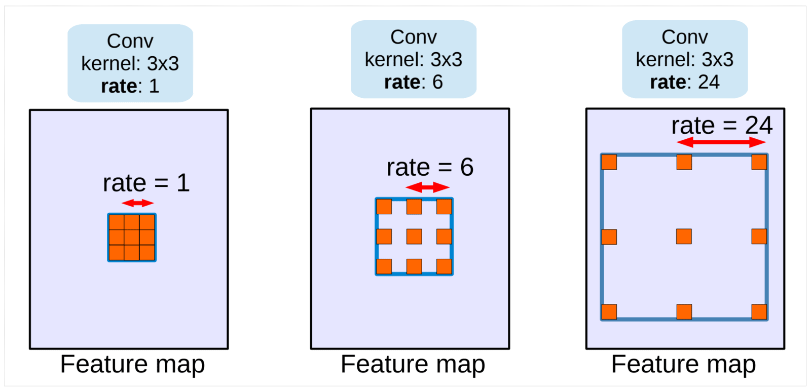
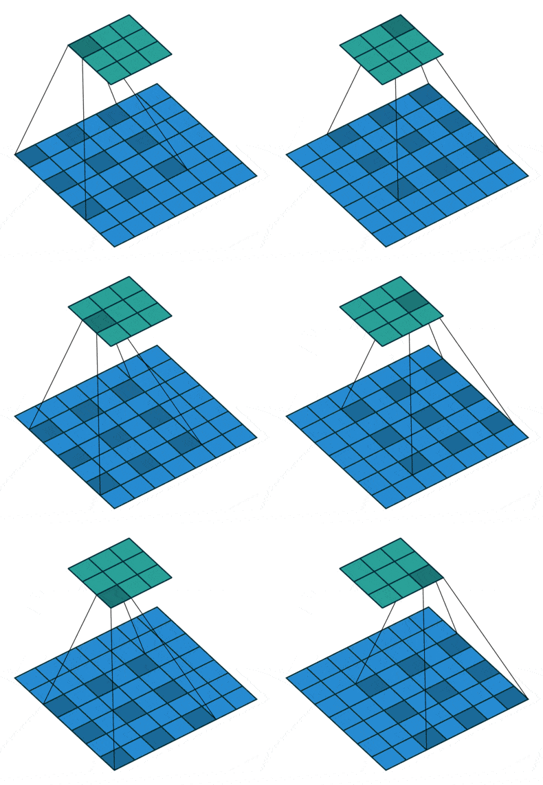
1. Atrous convolution, also known as dilated convolution, is a powerful technique actively used for segmentation tasks.
2. It allows us to control the resolution at which features are computed by the DCNN and adjusts the filter’s FOV to capture long-range information.
3. As indicated in the above diagram, dilation of convolutional kernels is equivalent to inserting holes (‘trous’ in French) between filter weights.
4. Using dilated convolution kernels, one can easily use the ImageNet pre-trained networks to extract denser feature maps. It can be easily applied to a trained network and seamlessly integrated during training.
5. Compared to regular convolution with larger filters, atrous convolution allows us to effectively enlarge the FOV of filters without increasing the number of parameters or the amount of computation.

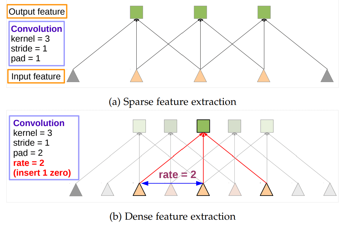
a) Sparse feature extraction with standard convolution on a low-resolution input feature map
b) Dense feature extraction with atrous convolution with rate r=2, applied on a high-resolution input feature map.

Mathematically, consider a two-dimensional signal. For each location i on the output y and a filter w, atrous convolution is applied over the input feature map x:

where the atrous rate r corresponds to the stride with which we sample the input signal. 

This is equivalent to convolving the input x with upsampled filters produced by inserting (r−1) zeros between two consecutive filter values along each spatial dimension.  

💡 Standard convolution is a special case where the rate: r=1.

Atrous Spatial Pyramid Pooling (ASPP)

As the name suggests, ASPP is simply SPP, but with atrous convolution. 

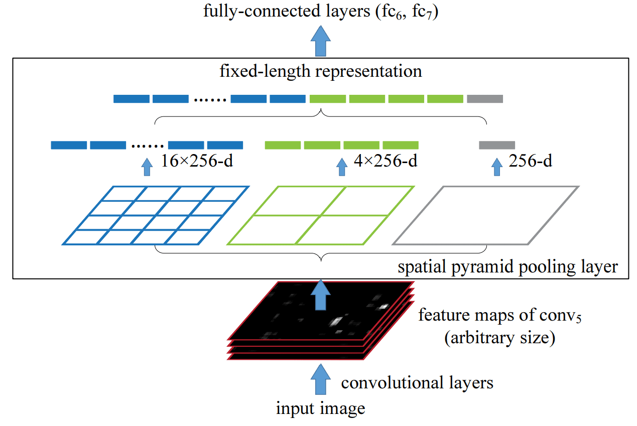
1. SPP was proposed as a replacement for the pooling layer to remove the fixed-size constraint of classification models.
2. The technique used in SPP proved that it is effective to resample features at different scales for accurately and efficiently classifying regions of an arbitrary scale.

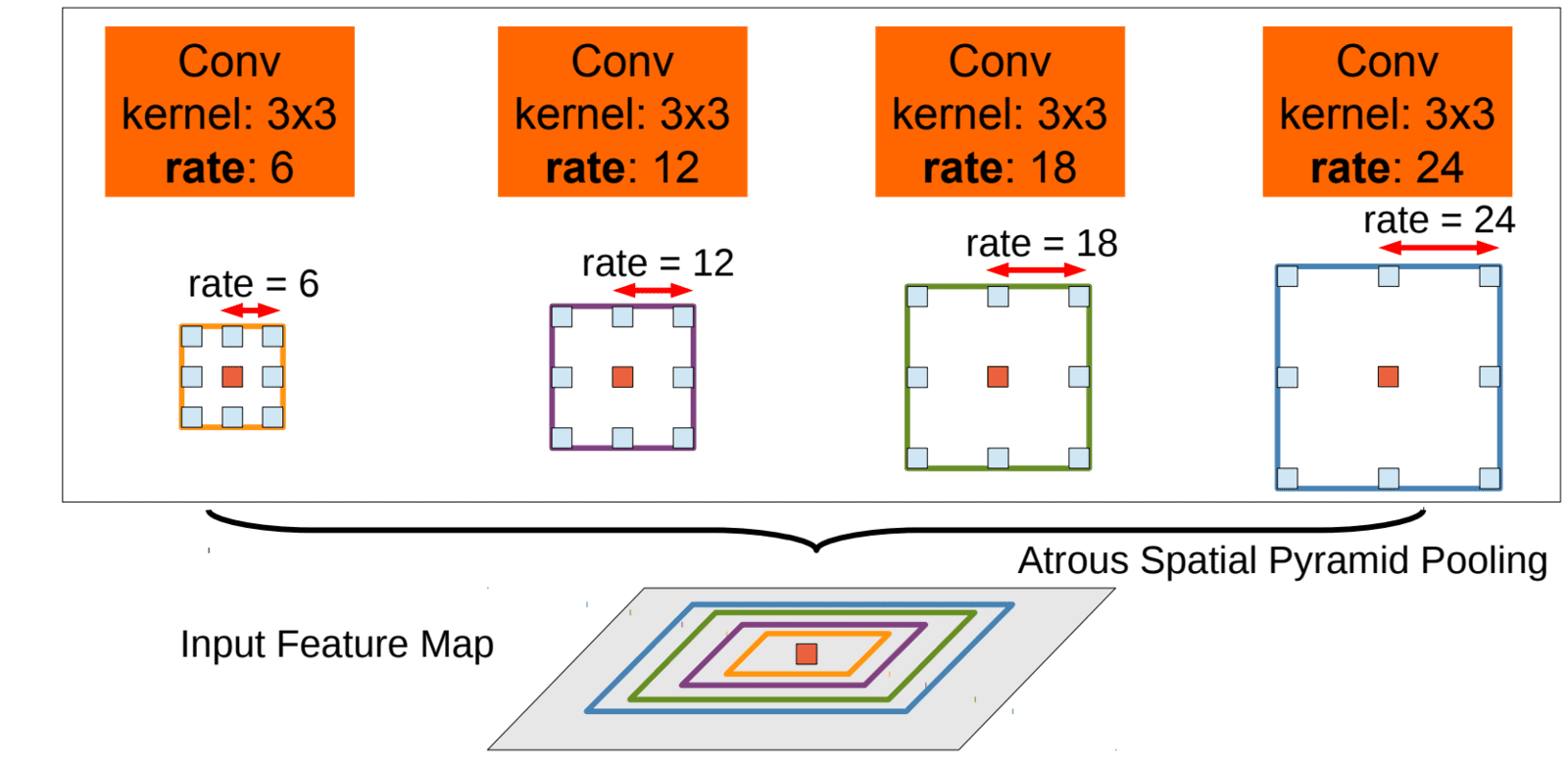
To classify the center pixel (orange), ASPP exploits multi-scale features by employing multiple parallel filters with different rates. The effective Field-Of-Views (FOV) are shown in different colors.

In light of the success of SPP in image classification and object detection, the authors proposed an ASPP module for semantic segmentation in DeepLabv2. Both v2 and v3 models use atrous convolution in SPP as a context module to incorporate multi-scale context to refine the feature maps.

1. The ASPP scheme employs multiple atrous convolutional layers in parallel.
2. Using different atrous rates amounts to probing the original image with multiple filters with complementary effective FOVs, thus capturing objects and valuable image context at multiple scales. 
3. The features extracted for each sampling rate are further processed in separate branches and fused to generate the final result.
   

But by using large and different atrous/dilation rates, the authors found a problem:

“As the sampling rate becomes larger, the number of valid filter weights (i.e., the weights applied to the valid feature region, instead of padded zeros) becomes smaller.”

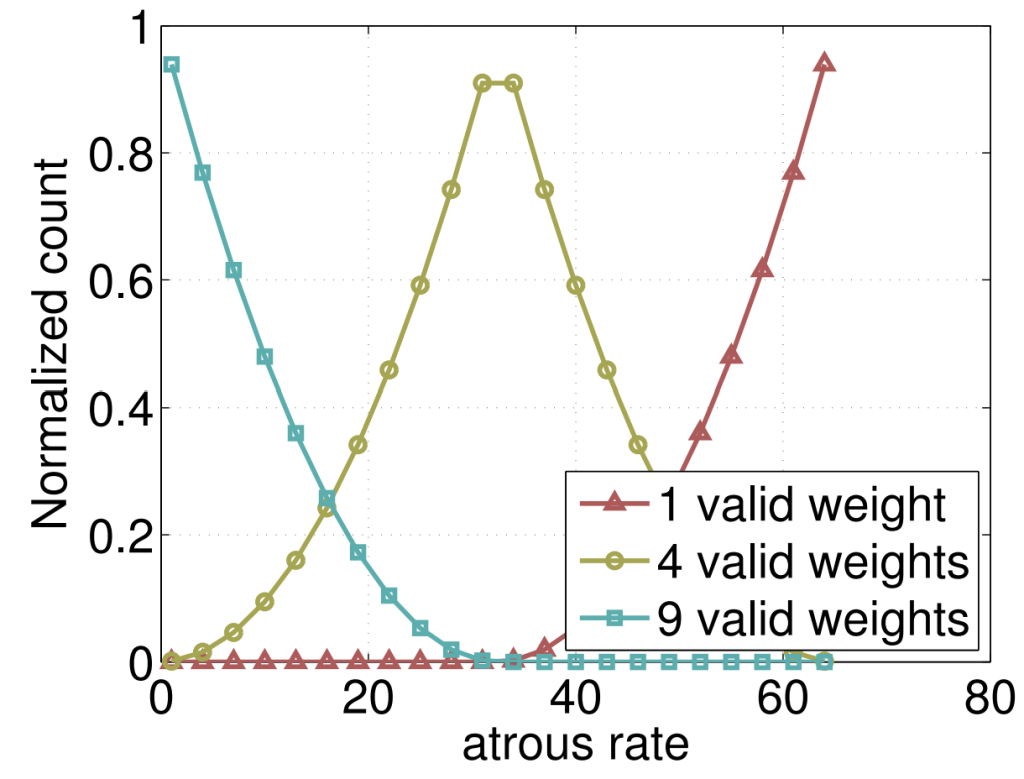
When a (3×3) filter is applied to a (65×65) feature map with different atrous rates. In the extreme case, where the rate_value≈feature_map size, the (3×3) filter, instead of capturing the whole image context, degenerates to a simple (1×1) filter since only the center filter weight is effective.  

DeepLabv3 Modifications To ASPP

The modifications made to the ASPP module used in DeepLabv3 are as follows:

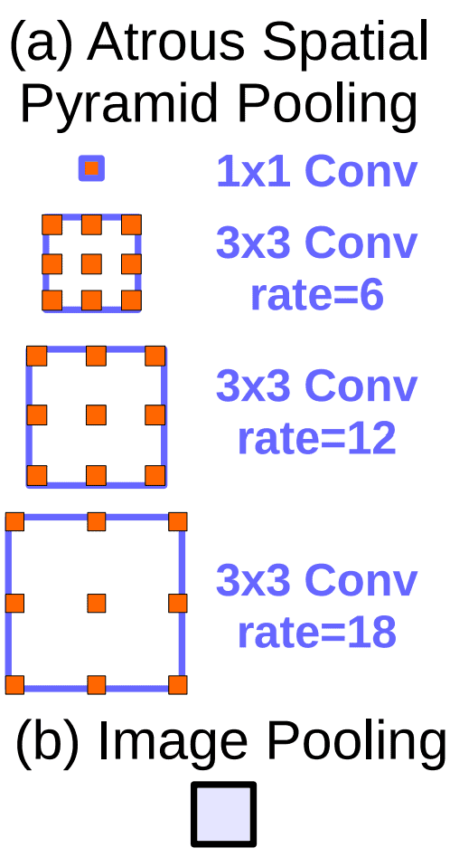
1. An “Image Pooling” module is added, which uses a global average pooling operation to encode global contextual information. This addition helps to alleviate the problems the model faces when using large dilation rates.
   
2. Use of batch normalization within ASPP. 
   
3. Use one (1×1) and three (3×3) convolutions. For (3×3) kernels, the dilation rate is set to (6, 12, 18) when the output stride is 16. For the output stride of 8, the dilation rates are doubled.
   
4. Each convolutional layer uses 256 output channels. Even the output from image pooling is first passed through a (1×1) convolutional layer to reduce the number of channels.
   
5. The resulting feature maps from all the branches are concatenated and passed through another (1×1, 256) convolution (and batch normalization) before generating final logits.

DeepLabv3 Architecture

As stated before, deep convolutional neural networks employed in a fully convolutional fashion are very effective but entail problems for semantic segmentation. For this, DeepLabv3 makes use of atrous convolutions.

The authors experimented with two design choices for dilated convolution in the paper:

1. By arranging several blocks using atrous convolution in a cascade.
2. Arranging atrous convolution blocks in parallel like SPP module – ASPP.

Atrous Convolution Arranged In A Cascade

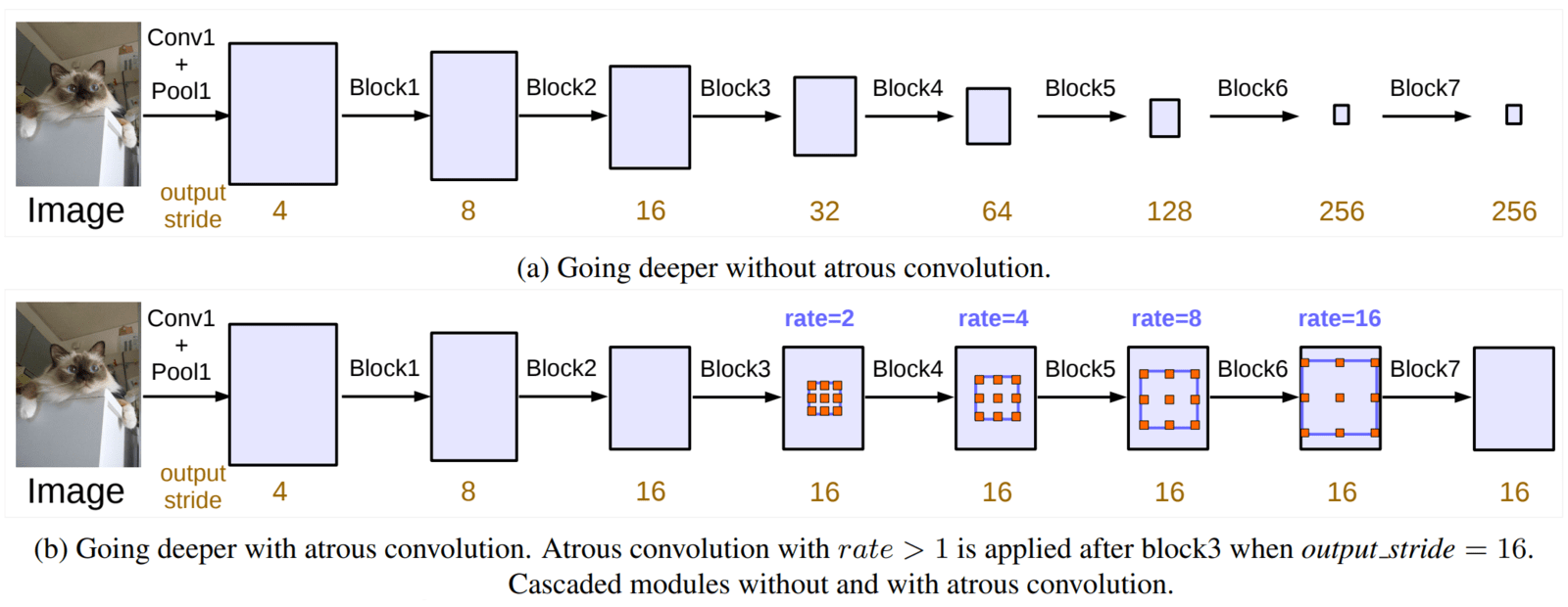
In the first design choice:

1. The last layer convolutional block (“conv5x”/layer4) from the ResNet backbone is copied and arranged three times, one after the other. In total, the backbone now has 7 blocks.
   
2. Each block (4-7) consists of three residual blocks (1×1, 3×3, 1×1). All except the last block uses a convolutional stride of 2 for downsampling.

In figure (a), with up to 7 cascaded ResNet blocks and image size 256, if no atrous convolution is applied, the output_stride (OS) changes from 32 to 256. The output_stride is the ratio of the spatial resolution of the input image to the final output resolution.

“The motivation behind this model is that the introduced striding makes it easy to capture long-range information in the deeper blocks. For example, the whole image feature could be summarized in the last small resolution feature map. However, we discover that the consecutive striding is harmful for semantic segmentation since detailed information is decimated.”

Fix: 

1. Atrous convolution is used with rates to get the desired output_stride of 16, figure (b). 
2. Change the convolution stride in block4 from 2 → 1 and the dilation rate to r=2. 
3. Similar changes are made to the rest of the blocks.

In this manner, the OS at block4 changes from 32 → 16. The subsequent blocks use larger atrous rates to extract denser feature maps at the same output_stride OS=16. 

Similarly, for an OS=8:

1. In block3, set convolutional stride=1 and dilation rate r=2. 
2. Consequently, in block4, along with setting convolutional stride=1, the dilation rate is set to r=4.

Experimental Results For Cascading Atrous Convolutions

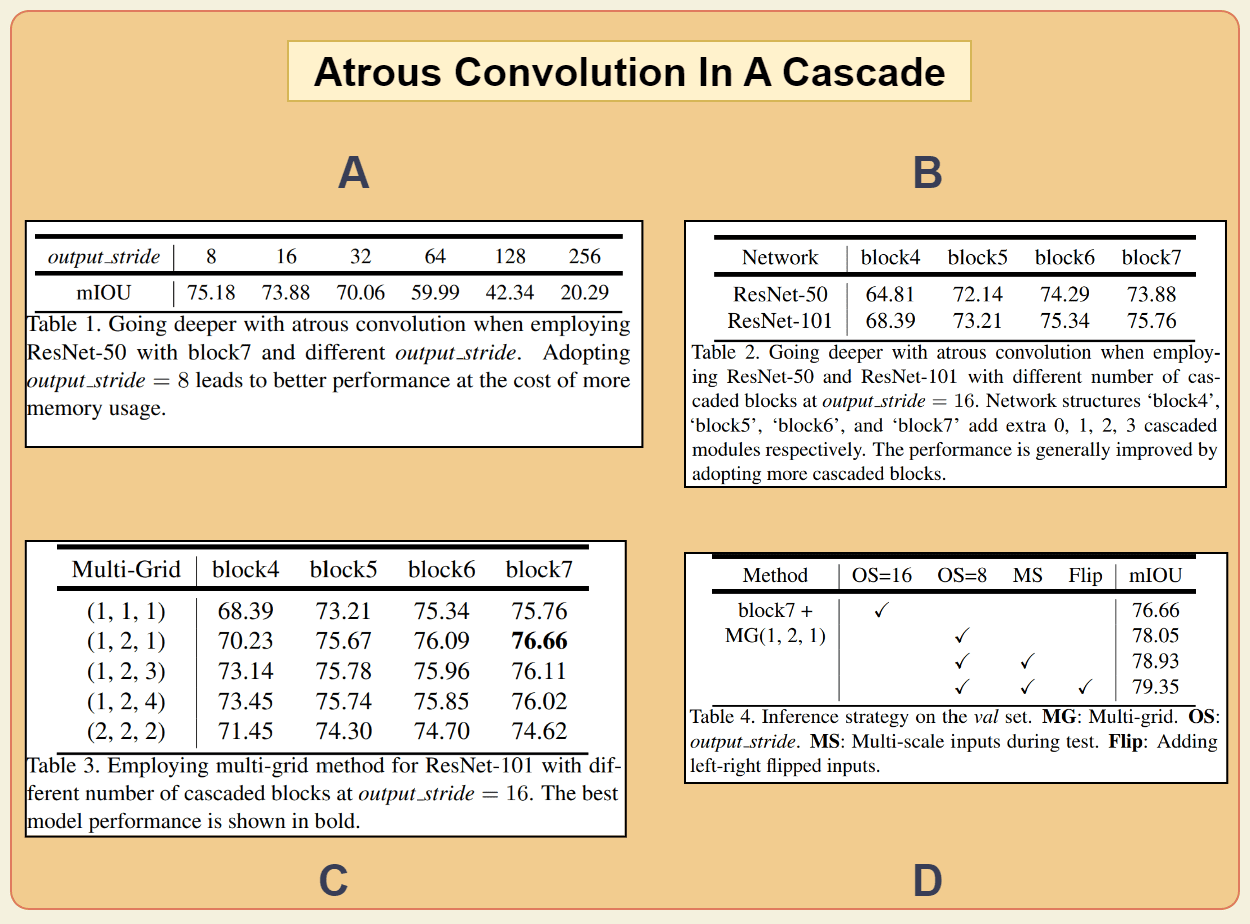
For the first design choice, the authors conducted several experiments, which they have outlined in the paper. Here, we’ll only discuss the methodology used in the final experiment that achieves the best result. This model design achieves an mIOU score of 79.35% on the Pascal VOC val set (table 4). 

These results were achieved using the following:

1. A 7-layer ResNet-101 backbone with atrous convolutions.
2. A multi-grid (MG) approach, i.e., using different atrous rates for the three convolutional layers in a block 4-7. The unit rates  (r1,r2,r3)=(1,2,1) are multiplied by the corresponding rate of the block.  E.g., The final dilation rate for block4 is,  final=2*(1,2,1)=(2, 4, 2).
3. Passing inputs during testing at multiple scales: {0.5, 0.75, 1.0, 1.25, 1.5, 1.75}.
4. Adding left-right flipped inputs.

🎯 mIOU stands for mean Intersection-over-Union, is a 🥇metric score used to determine the quality of predicted segmentation results.

Similarly, IOU is also used in object detection to quantify the quality of the predicted bounding boxes. Due to the weight of the topic, we’ve covered the use of Intersection over Union in Object Detection and Segmentation in-depth in a separate post.

Atrous Convolution Arranged In Parallel

The above figure illustrates the second design choice that the authors explored. Based on the empirical results and reduced FLOPS achieved using this design, the above architecture was selected and now represents the “DeepLabv3 semantic segmentation model”.

The architectural detail of this design are as follows:

1. It uses the ResNet-101 DCNN model as the backbone. When OS=8, the last two blocks (block3 and block4) contain atrous convolution with dilation rate=2 and rate=4, respectively. Whereas for OS=16, the dilation rate of just block4 is set to rate=2.
2. The output feature map from block4 is passed through the modified ASPP module. 
3. The outputs from all five sub-modules in the ASPP are concatenated and passed through the pen-ultimate (1×1) convolutional block. This block is for mixing the feature maps acquired by different sub-modules.
4. Finally, to generate predictions, the feature map passes through the final (1×1) convolution before being bilinearly upsampled depending on the OS.

Experimental Results For Atrous Convolutions In Parallel

Building up on the first design experiments, the authors use similar strategies for this design. The DeepLabv3 model achieves an mIOU score of 82.70% on the Pascal VOC Val set (table 6). Even without the extra COCO dataset, it beat the mIOU score (79.77%, +0.42%) set by the first design.

The authors first created a baseline model with a ResNet-101 backbone with OS=16 and with only the ASPP module. In subsequent experiments, they experiment with the MG unit rates and the image pooling module. 

The initial best result (Table 5) of 77.21% mIOU was obtained using:

1. A multi-grid with unit rates (1,2,4).
2. Using the dilation rate (6,12,18) for three (3×3) convolutions in ASPP.
3. Adding the global level context using image pooling.

Next, the authors apply the same inference strategy as the first design to the above model. In doing so, (Table 6) mIOU score increases to 79.77% (+2.56%).

Finally, by pre-training the model on the COCO dataset, the model achieved the best mIOU score of 82.70% on the Pascal VOC val set.

DeepLabv3 Results On The Pascal VOC Test Set

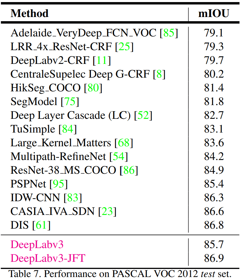
• The authors fine-tune the model on Pascal VOC 2012 “trainval” set.
  
• The batch normalization parameters are frozen, and use OS=8 for evaluating the test set.
  
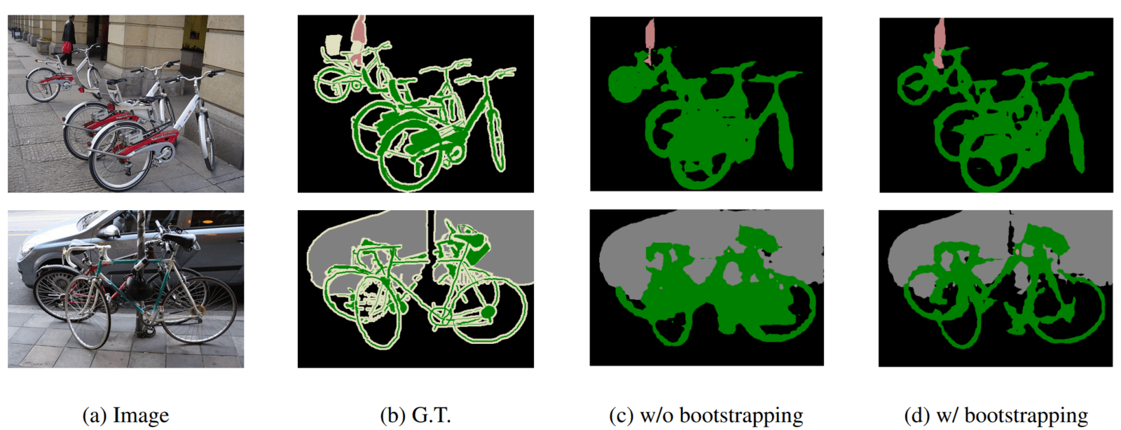
•  Using Bootstrapping: The images containing challenging classes in the training set are duplicated and used for training to improve scores further.
  
• Doing so,  DeepLabv3 achieved 85.7% on the Pascal VOC test set.
  
• Using the ResNet-101 model pre-trained on both ImageNet and JFT-300M datasets, the mIOU on the test set boosts 🚀 to 86.9% on the Pascal VOC test set.

Applications of Semantic Segmentation are endless. One such creative application is its use in background removal.

🐱‍👤 LearnOpenCV to the rescue.  We’ve tailored a post specifically for this, where we explain and perform foreground-background separation using semantic segmentation in Pytorch.

Going From DeepLabv3 To DeepLabv3+

The paper recognizes the benefits of two widely prominent techniques deep convolutional neural networks use for semantic segmentation tasks.

They are:

1. SPP or ASPP
2. Encoder-decoder structure

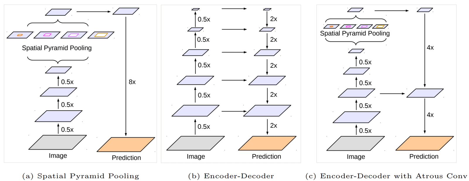
1. Networks that use SPP or ASSP modules can encode multi-scale contextual information by probing the incoming features with filters or pooling operations at multiple rates and multiple effective FOVs. ((a) DeepLabv3)
2. Even though the last feature map encodes rich semantic information, detailed information related to object boundaries is missing. 
3. Atrous convolutions could alleviate this by extracting denser feature maps. 
4. However, due to limited GPU memory, extracting and maintaining the output feature maps that are 8x (for 78 layers in ResNet-101) or even 4x times smaller is computationally prohibitive.
5. In this case, the (b) encoder-decoder models have the upper hand. The encoder can reduce the feature map resolution to capture long-range information. 
6. In the decoder path, the model can gradually recover the location/spatial information, such as object boundaries.
7. The proposed (c) DeepLabv3+ model uses the best of both worlds. With intermediate upscaling, concatenation, and processing blocks, the model has an OS=4.

DeepLabv3+ extends DeepLabv3 by adding a simple yet effective decoder module to refine the segmentation results, especially along object boundaries.

Components & Architecture Of DeepLabv3+

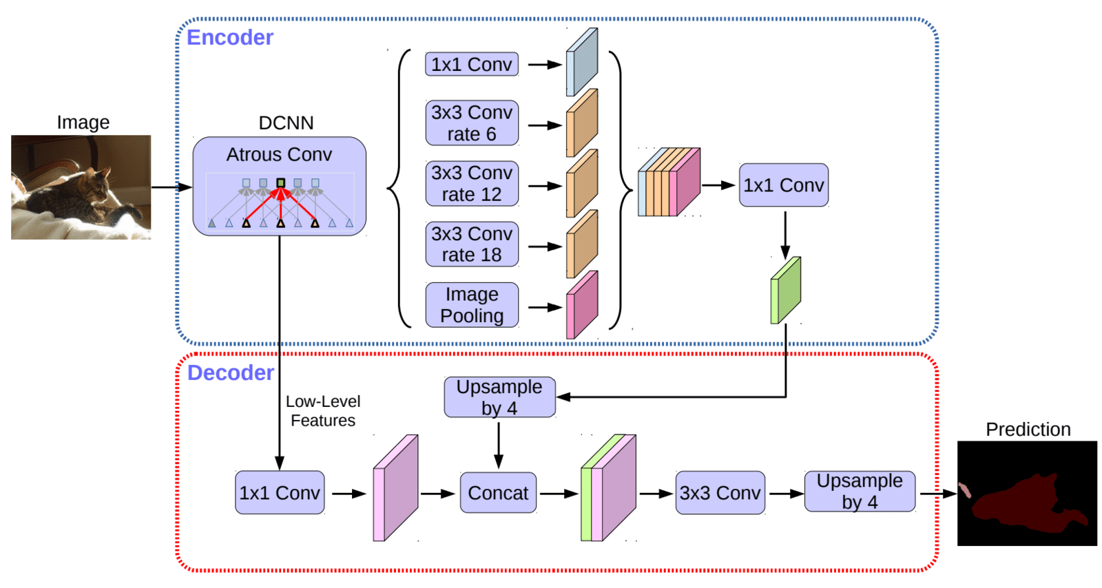
1. Backbone
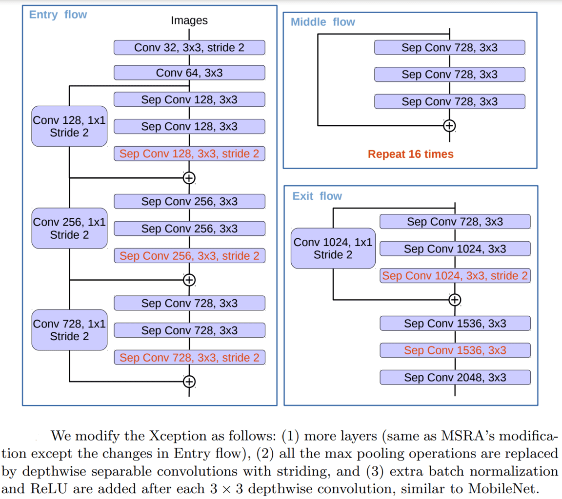
   • DeepLabV3+ employs a modified version of the “Aligned Xception” model as its primary feature extractor (backbone), further improving performance with faster computation. 
   • The modified backbone doesn’t update the “entry flow” like its counterpart, and all downsampling (max pooling) blocks are replaced with depth-wise separable convolutions. This allows the use of the proposed “atrous separable convolution” that helps to extract feature maps at an arbitrary resolution.
   • Batch normalization and ReLU activation layer follow each (3×3) depthwise separable convolution.
     
2. Encoder – DeepLabv3+ uses the DeepLabv3 model as the encoder. The output from the last feature map (before logits) is used as the input to the encoder-decoder structure.
   
3. Decoder
   1. DeepLabv3 usually outputs feature maps at an OS=16. This feature map is rich in semantic information. 
   2. Another feature map from the shallow layers (closer to the input) of the backbone is taken and subjected to (1×1) convolution to reduce the number of channels. This low-level feature map is rich in spatial information.
   3. The output from the encoder is first bilinearly upsampled by a factor of 4.
   4. Both feature maps from (1) and (2) are concatenated and passed through two (3×3) convolution blocks. 
   5. The merging allows the refinement of the encoder feature map with high spatial information (object boundary). 
   6. Finally, to generate predictions, the refined feature map is bilinear upsampling by a factor of 4. 

That’s all the details related to the architectural changes made to DeepLabv3+.

What Is Atrous Separable & Depthwise Separable Convolution?

In this section, we will briefly review “Atrous separable convolution” and how it differs from depthwise separable convolutions.

1. The MobileNet paper, back in ‘17, first introduced the depthwise separable convolution. 
2. The primary benefit is that it drastically reduces computation complexity with a tiny drop in accuracy, and being computationally efficient provides high inference speed on edge devices.
3. Depthwise separable convolution factorizes a standard convolution into two parts:
   
   1. Depthwise convolution – Performs a spatial convolution independently for each input channel.
   2. Pointwise convolution – Depthwise is followed by a pointwise (i.e., (1×1) convolution). Pointwise convolution is employed to combine the output from the depthwise convolution.

Atrous Separable convolution is simply depthwise convolution with dilation combined with pointwise convolution.

DeepLabv3+ Paper Experiments

In the DeepLabv3+, the authors have performed multiple experiments referring to the  Pascal VOC val set with different strategies and components. DeepLabv3+ also employs the same inference strategy as DeepLabv3.

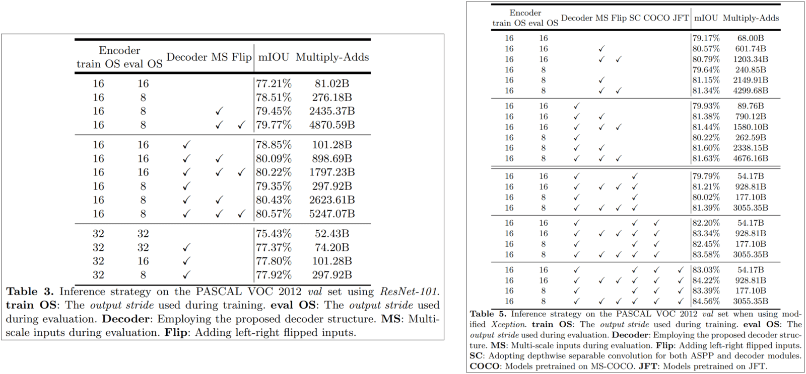
• First Row Block – No decoder
  • Shows the effect of using the modified Xception backbone. 
  • The authors report an improvement in the mIOU score from 79.17% → 81.34%.
  • With the same strategies, DeepLabv3 achieved the best score of 79.77%.

• Second Row Block: With the decoder
  • With only the decoder, the Xception backbone model jumps from 79.93% to 81.63% mIOU.
  • With the ResNet-101 backbone model lying behind.
    
• Third Row Block – Using depthwise separable convolutions in the ASPP and Decoder module.
  • This helps to reduce the number of Multiply-Adds operations by 33% to 41% while we still achieve results close to the original value.
  • It should be noted that even with depthwise separable convolutions, the mIOU of the Xception backbone is higher than that of the ResNet-101 backbone.
    
• Fourth Row Block – Pretraining on the COCO dataset
  • This boosts the results further by 2%.
    
• Fifth Row Block – Pretraining on the JFT dataset
  • Doing so, the scores are further improved by 0.8 – 1%.

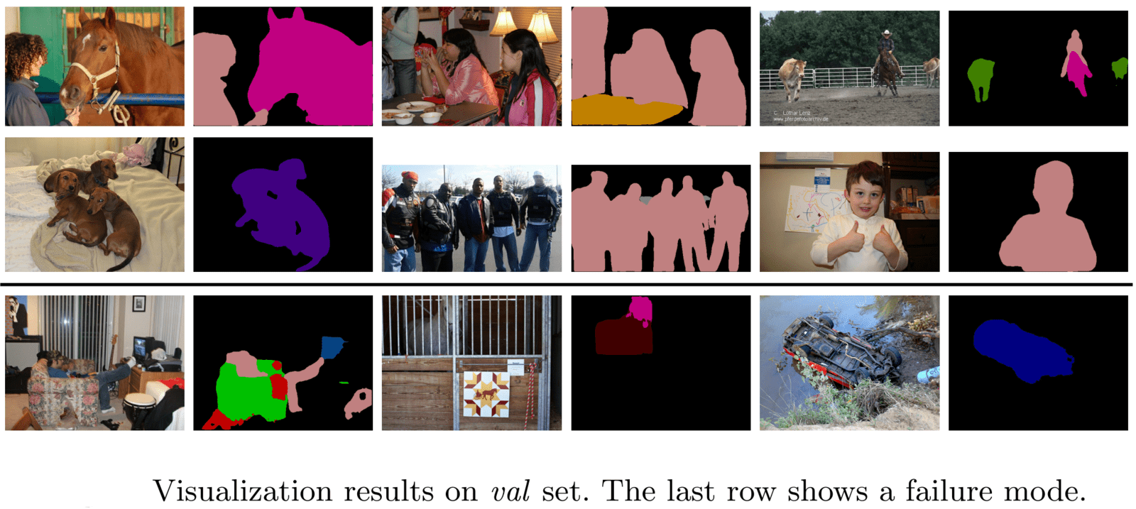
DeepLabv3+ On The Pascal VOC Test Set

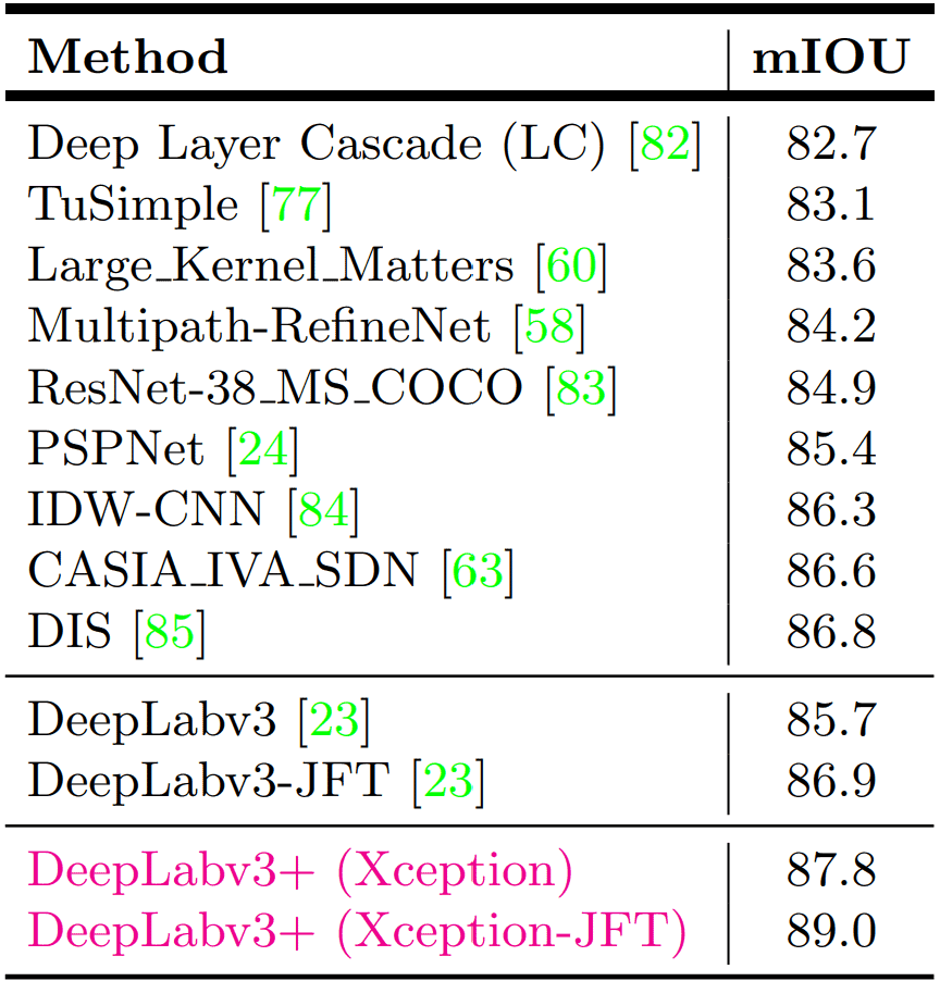
• The authors use the best model from the above experiments and train it with an OS=8 and frozen batch normalization parameters.
  
• In the end, DeepLabv3+ outperformed DeepLabv3 and several other top-performing models.
  
• DeepLabv3+ achieves an mIOU score of 87.8% and 89.0% without and with JFT dataset pretraining.

DeepLabv3+ On Cityscapes Test Set

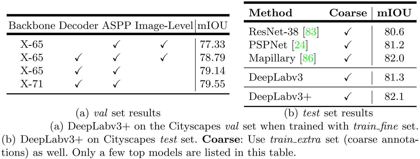
The Cityscapes dataset is a large-scale dataset containing high-quality pixel-level annotations of 5000 images (2975, 500, and 1525 for the training, validation, and test sets, respectively) and about 20000 coarsely annotated images.

• When trained (a) on the “train_fine” set, the authors used an Xception backbone with more layers and removed the“Image Pooling” module from the ASPP block.
• This results in an mIOU score of 79.55% on the val set.
• To compete with other SOTA models, the authors take the best model variant and fine-tune it using coarse annotations.
• Doing so (b), DeepLabv3+ achieved the SOTA mIOU score of 82.1% on the Cityscapes test set.
• This is significantly better than DeepLabv3.

To summarize, the contribution of DeepLabv3+ are:

• Use of encoder-decoder structure using DeepLabv3 as encoder and a simple and effective decoder.
• As the backbone and ASPP modules use atrous convolutions, one can easily control the extracted encoder feature map’s resolution to trade off precision and runtime. This is not possible by existing encoder-decoder models.
• Adapting Xception models for the segmentation task and using depthwise separable convolutions in both ASPP and decoder modules.

Semantic Segmentation Using DeepLabv3 in PyTorch

In this section, we’ll demonstrate how to load and perform inferences on the Pascal VOC 2012 val set.

Click here to download the source code to this post

The Pascal VOC dataset contains 20 object categories divided into 4 top-level classes.

• Person: person
• Animal: bird, cat, cow, dog, horse, sheep
• Vehicle: aeroplane, bicycle, boat, bus, car, motorbike, train
• Indoor: bottle, chair, dining table, potted plant, sofa, tv/monitor

Before we begin, you need to download and extract the Pascal VOC 2012 dataset.

I would recommend you first download the accompanying code for this blog post. Instead of downloading and extracting the dataset locally, we’ve provided a ready-to-go jupyter notebook that you can use on Google Colab.

We’ll first import the necessary modules.

# Necessary Imports
 
import os
import cv2
import PIL
import torch
import numpy as np
import matplotlib.pyplot as plt

Next, we define a variable label_map, that contains an RGB color tuple for each class, as in the above image.

label_map = np.array([
    (0, 0, 0),  # background
    (128, 0, 0),  # aeroplane
    (0, 128, 0),  # bicycle
    (128, 128, 0),  # bird
    (0, 0, 128),  # boat
    (128, 0, 128),  # bottle
    (0, 128, 128),  # bus
    (128, 128, 128),  # car
    (64, 0, 0),  # cat
    (192, 0, 0),  # chair
    (64, 128, 0),  # cow
    (192, 128, 0),  # dining table
    (64, 0, 128),  # dog
    (192, 0, 128),  # horse
    (64, 128, 128),  # motorbike
    (192, 128, 128),  # person
    (0, 64, 0),  # potted plant
    (128, 64, 0),  # sheep
    (0, 192, 0),  # sofa
    (128, 192, 0),  # train
    (0, 64, 128),  # tv/monitor
])

Next, we will define 2  utility functions to help process and plot the segmentation results.

• draw_segmentation_map(...) – This function is used for decoding the model outputs and each pixel’s RGB value depending on the predicted class.
• image_overlay(...) – This function performs weighted combinations of two images. It can be used for overlaying the segmentation maps on the raw image.

def draw_segmentation_map(outputs):
    labels = torch.argmax(outputs.squeeze(), dim=0).numpy()
 
    # Create 3 Numpy arrays containing zeros.
    # Later each pixel will be filled with respective red, green, and blue pixels
    # depending on the predicted class.
 
    red_map   = np.zeros_like(labels).astype(np.uint8)
    green_map = np.zeros_like(labels).astype(np.uint8)
    blue_map  = np.zeros_like(labels).astype(np.uint8)
 
    for label_num in range(0, len(label_map)):
        index = labels == label_num
        
        R, G, B = label_map[label_num]
 
        red_map[index]   = R
        green_map[index] = G
        blue_map[index]  = B
 
    segmentation_map = np.stack([red_map, green_map, blue_map], axis=2)
    return segmentation_map
 
 
def image_overlay(image, segmented_image):
    alpha = 1  # transparency for the original image
    beta  = 0.8  # transparency for the segmentation map
    gamma = 0  # scalar added to each sum
 
    image = np.array(image)
    segmented_image = cv2.cvtColor(segmented_image, cv2.COLOR_RGB2BGR)
    image = cv2.cvtColor(image, cv2.COLOR_RGB2BGR)
    
    cv2.addWeighted(image, alpha, segmented_image, beta, gamma, image)
 
    return image

Loading PyTorch DeepLabv3 Models

Key points to note:

• PyTorch provides three pre-trained DeepLabv3 variants. The varying factor over here is the backbone model.
• The three models are:
  • deeplabv3_mobilenet_v3_large(...) 
  • deeplabv3_resnet50(...)
  • deeplabv3_resnet101(...)
• These models were trained on a subset of COCO, using only the 20 categories in the Pascal VOC dataset.
• The images are trained with a minimum dimension size of 520.
• DeepLabv3 with mobilenet_v3_large backbone has an output_stride=16, whereas the DeepLabv3 with ResNet backbone has output_stride=8.
• One significant difference between the best models in the paper is the use of an atrous rate.
  • In the paper, excellent results were achieved using a multi-grid approach with unit rates (1, 2, 1).
  • However, the PyTorch models don’t follow these. Instead, for the resnet backbone model, it uses a dilation rate of r=2 across all (3×3) convolutional layers in block3/layer3 and a dilation rate of (2, 4, 4) for the three (3×3) convolutional layers in block4/layer4.
• A side note: ReLU activation function follows each batch normalization layer in ASPP and the penultimate (1×1) convolution layer.

The load_model(...) takes in the name of the backbone model to use and loads and returns the model along with the pre-processing transformations to be applied to use the model correctly.

from torchvision.models.segmentation import deeplabv3_resnet50, deeplabv3_resnet101, deeplabv3_mobilenet_v3_large
from torchvision.models.segmentation import (
                                             DeepLabV3_ResNet50_Weights, 
                                             DeepLabV3_ResNet101_Weights, 
                                             DeepLabV3_MobileNet_V3_Large_Weights
                                             )
 
def load_model(model_name: str):
    if model_name.lower() not in ("mobilenet", "resnet_50", "resnet_101"):
        raise ValueError("'model_name' should be one of ('mobilenet', 'resnet_50', 'resnet_101')")
        
    if model_name == "resnet_50":
        model = deeplabv3_resnet50(weights=DeepLabV3_ResNet50_Weights.DEFAULT)
        transforms = DeepLabV3_ResNet50_Weights.COCO_WITH_VOC_LABELS_V1.transforms()
 
    elif model_name == "resnet_101":
        model = deeplabv3_resnet101(weights=DeepLabV3_ResNet101_Weights.DEFAULT)
        transforms = DeepLabV3_ResNet101_Weights.COCO_WITH_VOC_LABELS_V1.transforms()
    
    else:
        model = deeplabv3_mobilenet_v3_large(weights=DeepLabV3_MobileNet_V3_Large_Weights.DEFAULT)
        transforms = DeepLabV3_MobileNet_V3_Large_Weights.COCO_WITH_VOC_LABELS_V1.transforms()
 
    model.eval()
 
    # Warmup run
    
    _ = model(torch.randn(1, 3, 520, 520))
    
    return model, transforms

In this article, we’ve only explored the possibility of using PyTorch for inference purposes. But that’s not it; we can also train DeepLabv3 models on custom datasets.

As such, quite recently, we published articles related to Automatic Document Scanning using OpenCV, where we first explored the possibility of using only traditional computer vision techniques. The document is first detected and segmented using Grabcut and returned after some post-processing.

But in hindsight, traditional segmentation methods (such as GrabCut) need to be calibrated to handle specific cases, and one can face great difficulty handling general cases. To tackle this, we need a deep learning-based semantic segmentation solution.

In the follow-up post, we first built a synthetic database of document images. Then by custom training DeepLabv3 in Pytorch on the artificial dataset, we overcame the shortcomings related to “document segmentation.”

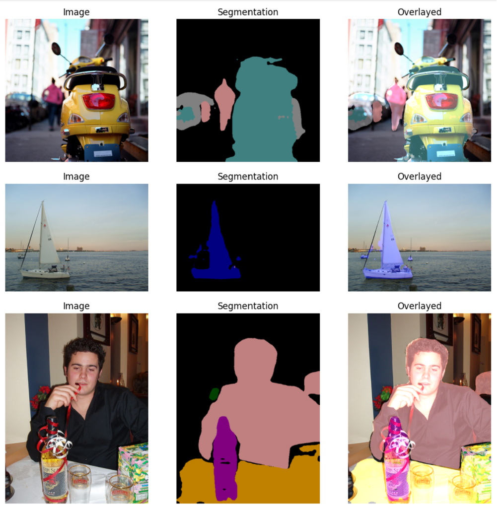
Next, we define one last function perform_inference(...) for:

1. Loading and preprocessing images
2. Model call
3. Post-process, plotting, and saving results.

def perform_inference(model_name: str, num_images=10, image_dir=None, save_images=False, device=None):
    
    if save_images:
        seg_map_save_dir = os.path.join("results", model_name, "segmentation_map")
        overlayed_save_dir = os.path.join("results", model_name, "overlayed_images")
        
        os.makedirs(seg_map_save_dir, exist_ok=True)
        os.makedirs(overlayed_save_dir, exist_ok=True)
    
    device = device if device is not None else ("cuda" if torch.cuda.is_available() else "cpu")
    model, transforms = load_model(model_name)
    model.to(device)
 
    # Load image handles for the validation set.
    with open(r"/content/VOCdevkit/VOC2012/ImageSets/Segmentation/val.txt") as f:
        val_set_image_names = f.read().split("\n")
 
    # Randomly select 'num_images' from the whole set for inference.
    selected_images = np.random.choice(val_set_image_names, num_images, replace=False)
 
    # Iterate over selected images
    for img_handle in selected_images:
        
        # Load and pre-process image.
        image_name = img_handle + ".jpg"
        image_path = os.path.join(image_dir, image_name)
        img_raw = PIL.Image.open(image_path).convert("RGB")
        W, H = img_raw.size[:2]
        img_t = transforms(img_raw)
        img_t = torch.unsqueeze(img_t, dim=0).to(device)
 
        # Model Inference
        with torch.no_grad():
            output = model(img_t)["out"].cpu()
 
        # Get RGB segmentation map
        segmented_image = draw_segmentation_map(output)
 
        # Resize to original image size
        segmented_image = cv2.resize(segmented_image, (W, H), cv2.INTER_LINEAR)
        overlayed_image = image_overlay(img_raw, segmented_image)
        
        # Plot
        plt.figure(figsize=(12, 10), dpi=100)
        plt.subplot(1, 3, 1)
        plt.axis("off")
        plt.title("Image")
        plt.imshow(np.asarray(img_raw))
 
        plt.subplot(1, 3, 2)
        plt.title("Segmentation")
        plt.axis("off")
        plt.imshow(segmented_image)
 
        plt.subplot(1, 3, 3)
        plt.title("Overlayed")
        plt.axis("off")
        plt.imshow(overlayed_image[:, :, ::-1])
        
        plt.show()
        plt.close()
 
        # Save Segmented and overlayed images
        if save_images:
            cv2.imwrite(seg_map_save_dir, segmented_image[:, :, ::-1])
            cv2.imwrite(overlayed_save_dir, overlayed_image)
 
    return

Finally, we can perform inference by executing the following lines:

ROOT_raw_image_directory = r"/content/VOCdevkit/VOC2012/JPEGImages"
 
model_name = 'resnet_50' # "mobilenet", "resnet_50", resnet_101
num_images = 4
save = False
 
perform_inference(
    model_name=model_name, 
    num_images=num_images, 
    save_images=save, 
    image_dir=ROOT_raw_image_directory
)

In the end, you should get outputs like these:

Summary

In this article📜, we covered a comprehensive list of related topics. To summarise:

1. We began by exploring the “DeepLab system” to answer the question, “what is DeepLabv3?”
2. We analyzed some common problems in segmentation tasks and their solution used in DeepLabv3.
3. We explored the two core components of DeepLabv3.
4. We took an exploratory route to understand the intuition behind the DeepLabv3 architecture backed by empirical results.
5. Next, we begin to investigate DeepLabv3+ and the intuition behind it.
6. We then explored the DeepLabv3+ architecture, specifically the new decoder.
7. We examined the critical results published in the DeepLabv3+ paper and how it faired compared to DeepLabv3.
8. Finally, we showed how easily we could use the DeepLabv3 models in PyTorch to perform inference on the Pascal VOC dataset.

We would love to hear from you. Please feel free to ask questions in the comment section; we are more than happy to converse with you.

References

1. DeepLabv3 paper – Rethinking Atrous Convolution for Semantic Image Segmentation
2. DeepLabv3+ paper – Encoder-Decoder with Atrous Separable Convolution for Semantic Image Segmentation
3. PyTorch for Beginners: Semantic Segmentation using torchvision
4. PyTorch Deeplabv3 documentation
5. Pascal VOC 2012 Challenge

🌟Happy learning!