Image Captioning using ResNet and LSTM

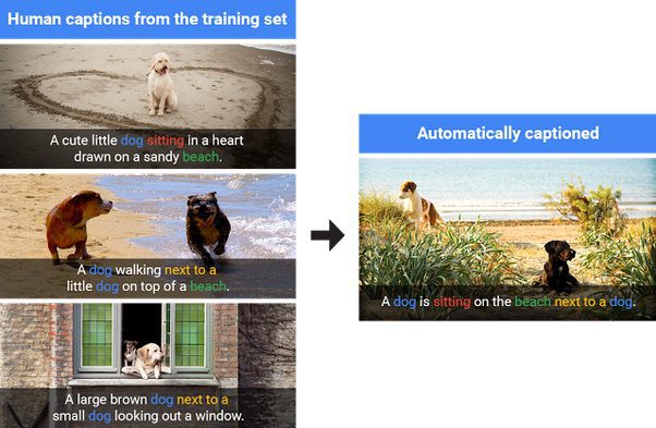
Imagine you’re watching a travel vlog on YouTube, and you turn on the image captions feature. As the video shows a stunning view of Mount Fuji, a caption appears: “Snow-capped Mount Fuji at sunrise with cherry blossoms in the foreground.” How does YouTube understand the visuals and generate such detailed descriptions? That’s the magic of image captioning.

Image captioning has gained a lot of attention in the machine-learning community over the past few years. The idea is remarkably intuitive-train a model to look at an image and output a relevant and coherent sentence that accurately describes it. It’s basically bridging the world of computer vision and natural language processing. Traditional computer vision tasks might focus on object classification, detection, or segmentation, while language models handle the complexities of generating and understanding human-like sentences. What if we put these together, and you have an end-to-end pipeline that “sees” images and “writes” short descriptions?

In this article, we will learn how to use ResNet (the CNN) as the eye and LSTM (the RNN) as the mouth of our machine so it can generate captions from images, like how we think about an image description after seeing it. Sounds interesting? Grab a cup of coffee, and let’s get started!

But wait, this is not the END!
We will provide training and inference scripts for you to explore the ResNet + LSTM fusion with your images to generate some decent captions! 

Applications of Image Captioning – Why do we need it?

All the image captioning applications work on a simple logic: “A picture may be worth a thousand words, but sometimes it’s the words that are most useful.” When we create captions, we often include unnecessary adjectives that a computer doesn’t need to understand the image. Instead, machines focus on extracting only the relevant context, which not only saves memory but also makes the captions more practical for various applications. A short, concise caption is more efficient and effective, as it avoids lengthy descriptions that aren’t useful when working with the data, ensuring better performance and resource optimization.

Before getting into the technical details, it’s important to understand why image captioning is useful. A system that can describe an image, such as “Two elephants standing near a tree in a savannah,” is more than just a “cool” technology. It has practical applications in various fields:

1. Accessibility for Visually Impaired People
   Screen readers do a great job reading text. However, images are a big part of our digital world, and they remain inaccessible if they do not contain alternate text. Image captioning helps by automatically generating text descriptions. So assistive technologies can read them out loud, making the web more inclusive for everyone.
2. Social Media and Photo Organization
   We constantly upload pictures on social platforms like Instagram, Facebook, or personal cloud galleries. Manually tagging or describing thousands of images is very hard and time-consuming. Automated image captioning can help by providing a textual description so you can search through your library effectively. Instead of searching “beach,” you could rely on a system that has automatically tagged all your beach photos as “People relaxing on a sandy beach.”
3. Content-Based Image Retrieval and SEO
   If you have a massive image database—think of stock photo sites—users might want to search for “man with sunglasses on a boat at sunset.” With automated image captions, your search engine can match textual queries to the descriptions generated for each photo. Platforms like Google use a similar approach, where captions or alt text, whether added manually or generated automatically, are stored as metadata. This metadata not only helps with image retrieval but also improves SEO by making the content more accessible and searchable.
4. Robotic Systems and Navigation
   Robots that move around in real-world environments often rely on cameras for vision. If these cameras can interpret the scene and generate textual or structured descriptions of what they see, the robot can make more informed decisions. For instance, “Hallway is blocked by a box” is a simple but crucial piece of information for navigation.
5. Online Marketing and E-commerce
   For e-commerce platforms, product images are a big deal. Automated captions describing product attributes can enhance SEO and streamline product cataloging.

Condensing the above use cases into a single sentence – Image captioning can help build more accessible platforms, aid content discovery, and supercharge search and recommendation engines.

Architecture Overview – Core Components of Image Captioning 

An image captioning system typically contains two components:

• Using a convolutional neural network (ResNet in our case) to extract visual features from the image.

• Decoding these features into a natural language sequence using a modified recurrent neural network (LSTM). 

Among CNNs, ResNet (Residual Neural Network) is a strong candidate for extracting relevant features. Meanwhile, an LSTM (Long Short-Term Memory) network is a common choice for handling the language generation because it can manage long-term dependencies in language sequences.

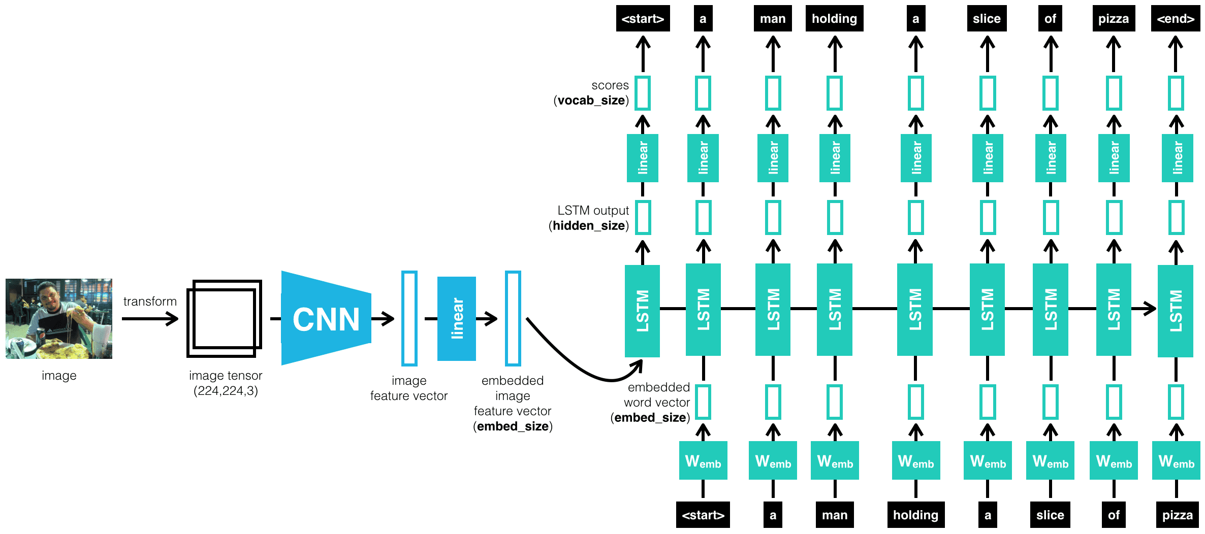
We’ll focus on the classic pipeline: a pre-trained ResNet feeding its visual features into an LSTM. Let’s understand how both the models individually contribute to the final architecture of image captioning.

ResNet 

ResNet was introduced by Kaiming He and colleagues back in 2015. The core idea was to let the network learn residual functions rather than direct mappings. Residual blocks have these “skip connections” that allow gradients to flow more effectively, solving the vanishing gradient problem that plagued very deep networks.

Where It Started?

It all began with the simple task of approximating a linear function, Y = Wx + b – the foundation of neural networks. We started with basic layers, updating weights and parameters through a process involving forward passes and backpropagation. This was groundbreaking, but then researchers wondered: Could we do the same for images? Could we teach a model to learn features through convolution?

Convolutional Neural Networks (CNNs) were born. For a while, these networks brought incredible breakthroughs, starting with AlexNet in 2012. AlexNet proved that stacking more layers—building deeper CNNs—could dramatically improve image recognition. The success has led to even more complex architectures like VGG and GoogleNet.

But as we stack more layers, a new problem emerges: vanishing and exploding gradients. Simply put, the deeper these networks went, the harder it became to train them. Gradients would either fizzle out to near-zero or explode to massive values, causing performance to degrade unpredictably.

Then, in 2015, ResNet arrived to rewrite the rules. Kaiming He and his colleagues introduced residual learning, a clever approach that changed everything. With a simple yet powerful trick – the skip connection – ResNet made it possible to train networks with hundreds, even thousands, of layers. This breakthrough shattered previous limitations and opened new doors for deep learning, proving that deeper could indeed be better.

The Residual Network

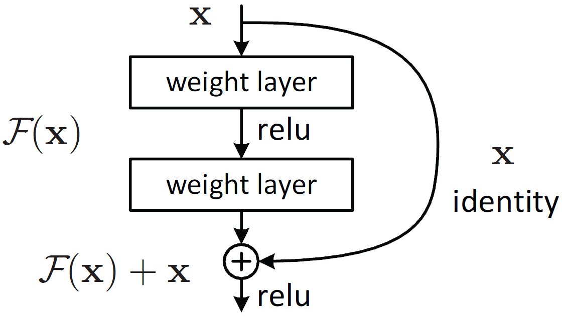
ResNet, short for Residual Network, introduced the concept of residual blocks to overcome the limitations of traditional deep architectures. The key innovation lies in its skip connections—shortcuts that bypass certain layers, allowing the model to learn residual mappings instead of directly optimizing for the target function. Mathematically, this is represented as 

F(x) = H(x) − x

H(x) is the desired mapping, and F(x) represents the residual. Adding x back at the output yields H(x) = F(x) + x. This approach ensures gradients flow smoothly during backpropagation, mitigating vanishing gradients. By stacking these blocks, ResNet achieved a top-5 error rate of 3.57% and won first prize in the ILSVRC classification competition in 2015.

Why ResNet for image captioning?

Fast-forward to image captioning-where we want a neural network to look at an image and tell us what it sees. This needs a power vision feature extractor. We feed an image into a CNN to extract the most important visual cues. Since ResNet is known for its strong, robust representations–many captioning architectures choose it as their backbone. It sees the picture and extracts high-level features, which are then fed to the decoder (e.g., an LSTM). Finally, the decoder generates a sequence of words representing the content in the image.

LSTM

Next up is the LSTM, a type of recurrent neural network (RNN) that helps us tackle the problem of generating sequences (in this case, textual descriptions of images).

Why not RNNs?

Many tasks require us to handle sequential information, such as predicting the next word in a sentence or determining actions over time. Classic neural networks process inputs as independent data points, ignoring context from past inputs. Recurrent Neural Networks (RNNs) solve this by having “loops” that pass along hidden states across time steps. This allows the model to keep a form of memory, so each new prediction can depend on what was previously seen. But standard RNNs struggle with long-term dependencies: if an event happened many steps ago, the network might forget or distort that information. This leads to vanishing or exploding gradients during training, which hinders their ability to learn when sequences stretch out over many time steps.

LSTM at a Glance

Long Short-Term Memory (LSTM) addresses the vanishing/exploding gradient issue by introducing a memory cell and a set of gating mechanisms. Let’s imagine a sequence like, “I grew up in France… I speak fluent French.” By the time we see “French,” we want the network to recall “France” from earlier. 

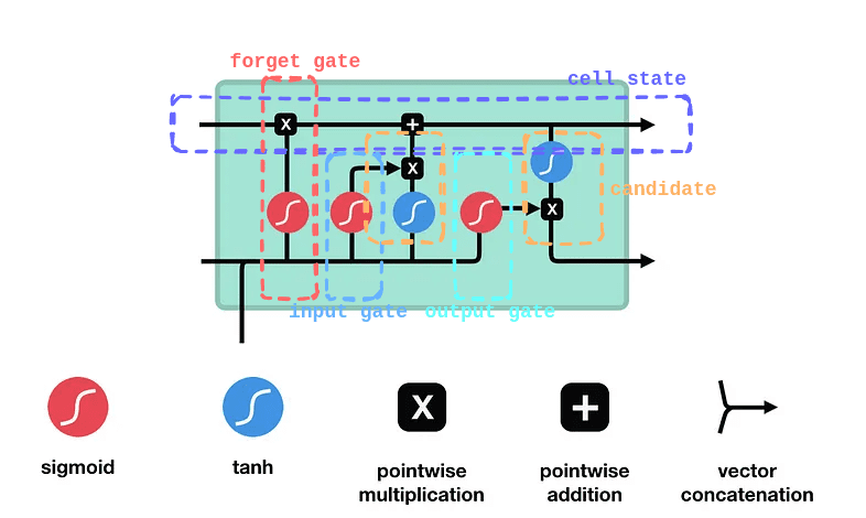
LSTM’s internal structure lets it keep or discard certain details across time, allowing it to handle long-term dependencies effectively. It achieves this through four core components: the forget gate, input gate, cell state, and output gate. Each component plays a crucial role in deciding what information to retain, update, or pass forward, ensuring that relevant context is maintained throughout the sequence.

Forget Gate

The forget gate decides which parts of the previous cell state to erase. For example, once the sentence shifts from talking about “growing up in France” to the subject, “I speak…,” the LSTM might retain the “location = France” fact but forget unrelated details from earlier words. It multiplies the old cell state by a factor (0 to 1) based on the current input and past hidden state.

Input Gate

The input gate controls how much new information enters the cell state. If we see the word “fluent,” the input gate determines how strongly that feature updates the memory cell. Another mini-network simultaneously creates a “candidate” vector that represents what could be added (like “fluent => language skill”). The input gate then scales this candidate, deciding how much to actually write into memory.

Candidate Cell Update

Although not always called a separate “gate,” this is the step where the LSTM adds fresh content to the cell. The forget gate has already cleared unnecessary info, and the input gate decides how much of the new candidate to store. So if the network identifies that “France” plus “fluent” suggests a strong possibility of “French,” it stores that as an updated piece of knowledge in the memory cell.

Output Gate

Finally, the output gate decides what to “expose” as the hidden state for the current time step. It reads the updated cell, applies a filter (0 to 1), and passes along only relevant parts-like the notion that “French” is the likely language reference. This hidden state is then sent forward to help predict the next word or feed the next step’s gates.

Through backpropagation, the model learns how to scale these gates for each word. Over time, it discovers when to retain useful facts (e.g., “France” is relevant for “French”) and when to discard extras.

Connecting Features to LSTM

Often, we feed features (vectors representing our data at each time step) into an LSTM to predict a series of outputs or to generate a final prediction. These features can come from raw embeddings (like word embeddings in a language model) or from other networks (like a CNN that extracts visual features). At each time step, the LSTM receives the current feature vector and its own hidden state from the previous step. The gates update the memory cell, and the LSTM outputs a hidden state that reflects both the recent features and the long-range context. This method is effective in many domains-language modeling, speech recognition, and image captioning because it balances short-term updates with the ability to preserve long-term signals.

But Why Are We Using ResNet and LSTM for Image Captioning Today?

You might be thinking: “Transformers are the new big thing. Why do we need ResNet and LSTM?” That’s a fair question. VLMs (Vision Language Models) powered by Transformers and attention-based mechanisms have indeed set new benchmarks in text and even in image captioning. However, ResNet+LSTM, a classic pipeline that is proven, well-documented, and relatively straightforward to implement, can act as a building block for learning the concepts of image captioning.

Educational Purposes
For someone stepping into the world of deep learning-based captioning, starting with ResNet+LSTM helps build an intuitive understanding of how CNNs connect to RNNs. Transformers can feel a bit more abstract and complicated if you haven’t tackled simpler architectures first.

Resource Requirements
Transformers usually require large-scale data and compute to train properly. They might also be overkill if you just want a simple demonstration or a smaller-scale system. A well-tuned ResNet+LSTM can get decent results without monstrous computational resources.

Backbone for Modern Architectures
Despite the emergence of newer models, ResNet and LSTM continue to serve as foundational backbones in many advanced architectures. Architectures like Attention OCR, YOLO, and hybrid models combining transformers with CNN backbones often rely on ResNet (the skip connection method) for feature extraction. Similarly, LSTM remains a go-to choice for sequence modeling applications like video classification, text recognition, and caption generation.

Performance on Standard Benchmarks
ResNet+LSTM models can still hold their accuracy on some smaller or mid-level datasets, providing a good performance/complexity trade-off. So, while the world is definitely embracing attention-based models, ResNet+LSTM is still relevant and offers a great stepping stone.

Click here to download the source code to this post

Code Pipeline – How Image Captioning Works in Code?

Now, let’s try to implement the logic in code, the fun part. We aim to illustrate how each piece of code fits together and what happens under the hood. We will work with two code files, 

train.py – A Jupyter Notebook containing the training code.

app.py – An inference script to test the trained model on images.

Interesting right? Let’s start.

Overview of Code Pipeline of Image Captioning

1. Vocabulary: Build a word vocabulary from the captions (text).
2. Dataset: Load the Flickr8k images and captions, apply transforms, and prepare the data for training.
3. Encoder (ResNet): Convert images into feature vectors.
4. Decoder (LSTM): Generate captions word-by-word from the feature vectors.
5. Training: Combine the encoder & decoder, compute loss, and optimize.
6. Inference: A Gradio interface to run the inference with our trained model.

We’ll go through each part in detail.

Imports and Configuration

Let’s start with the imports and initial configuration.

import os
import re
import csv
import pickle
import torch
import torch.nn as nn
import torch.optim as optim
from torch.utils.data import Dataset, DataLoader
import torchvision.transforms as transforms
import torchvision.models as models
from torchvision.models import ResNet50_Weights
from collections import Counter
from PIL import Image
import numpy as np
import random

from tqdm import tqdm

Core Modules:

os, re, csv, pickle for file handling, text processing, reading CSV files, and saving/loading serialized data.

PyTorch:

torch, torch.nn, torch.optim core PyTorch library for defining models, layers, loss functions, and optimization.

torch.utils.data provides Dataset and DataLoader utilities for creating and iterating over datasets.

TorchVision:

transforms for preprocessing images (e.g., resizing, normalization). models pretrained models, like ResNet-50.

ResNet50_Weights provides default weights for ResNet-50.

Other Libraries:

Counter for counting occurrences of words during vocabulary building.

PIL.Image for image manipulation. numpy for numerical operations.random: For shuffling data.

tqdm for progress bars during training.

EMBED_DIM = 256
HIDDEN_DIM = 512
LEARNING_RATE = 0.001
BATCH_SIZE = 64
EPOCHS = 50
MIN_WORD_FREQ = 1
SEED = 42
DEVICE = torch.device("cuda" if torch.cuda.is_available() else "cpu")
NUM_WORKERS = 4

IMAGES_DIR = "flickr8k/Images"
TOKENS_FILE = "flickr8k/captions.txt"

BEST_CHECKPOINT_PATH = "best_checkpoint.pth"
FINAL_MODEL_PATH = "final_model.pth"
VOCAB_PATH = "vocab.pkl"

RESUME = False

EMBED_DIM refers to the dimensionality of the vector space where features or tokens are embedded. It defines the size of the feature representation extracted by the encoder or used in the decoder, balancing between the expressiveness of the features and computational efficiency. A value like 256 ensures a good trade-off between detail and performance.

HIDDEN_DIM is the size of the hidden states in the LSTM decoder, determining how much information the model can store and process over time. A higher dimension like 512 allows for better capacity to capture long-range dependencies in sequences, which is crucial for tasks like caption generation.

LEARNING_RATE is the step size for updating model weights during optimization. It controls how much the model learns from the gradient at each step. A value of 0.001 is commonly chosen as a starting point to ensure stable convergence without overshooting the minimum loss.

BATCH_SIZE specifies how many samples are processed together in one forward and backward pass. A batch size of 64 strikes a balance between computational efficiency and the stability of gradient updates, leveraging parallelism in modern hardware.

EPOCHS defines the number of times the entire training dataset is processed. Training for 50 epochs ensures sufficient updates to the model weights while avoiding overfitting or unnecessary computation.

MIN_WORD_FREQ sets the threshold for filtering out infrequent words during vocabulary creation. Words appearing less than this threshold are treated as unknown, reducing noise in the dataset while maintaining meaningful vocabulary coverage.

SEED ensures reproducibility by fixing the initialization of random processes in libraries like PyTorch, NumPy, and Python’s random. Setting it to 42 is a conventional choice and allows experiments to be consistently replicated.

DEVICE determines whether the computations are performed on a GPU or CPU. Using torch.device(“cuda”) when a GPU is available speeds up training significantly, while falling back to CPU ensures compatibility.

NUM_WORKERS specifies the number of parallel processes used to load data during training. With a value of 4, data loading is efficient without overloading the system resources, improving throughput.

Paths like IMAGES_DIR and TOKENS_FILE indicate where the dataset (images and captions) is stored, ensuring the code knows where to retrieve necessary files. BEST_CHECKPOINT_PATH and FINAL_MODEL_PATH define locations for saving model weights, the former for intermediate checkpoints to recover from interruptions and the latter for the final, fully trained model. VOCAB_PATH is where the vocabulary is stored, encapsulating the mapping of words to indices for efficient data processing.

Lastly, the RESUME flag controls whether training resumes from a saved checkpoint or starts afresh. This is particularly useful in scenarios where training is interrupted or when fine-tuning is desired. Together, these parameters ensure a structured and reproducible training pipeline.

random.seed(SEED)
np.random.seed(SEED)
torch.manual_seed(SEED)

These lines set the random seed for Python, NumPy, and PyTorch to ensure that results are reproducible. This means shuffling, initialization, and other random operations will produce the same results every time the code is run.

Vocabulary Class

The Vocabulary class is a crucial component in Natural Language Processing (NLP) tasks, especially in image captioning, as it bridges the gap between raw text and numerical data that the model can process. This class is designed to tokenize text, build a vocabulary, and convert words into numerical representations. Let’s break it down in detail.

class Vocabulary:
    def __init__(self, freq_threshold=5):
        self.freq_threshold = freq_threshold
        self.itos = {0: "pad", 1: "startofseq", 2: "endofseq", 3: "unk"}
        self.stoi = {v: k for k, v in self.itos.items()}
        self.index = 4    def __len__(self):        return len(self.itos)

The __init__ method initializes the vocabulary with a freq_threshold, which specifies the minimum frequency a word must have to be included. Words appearing less often than this threshold are mapped to a special token like unk (unknown). By default, freq_threshold is set to 5, ensuring the vocabulary focuses on common words, reducing noise and memory usage. The itos dictionary maps indices to special tokens (pad, startofseq, endofseq, unk), which serve specific purposes, like padding sequences, marking the beginning or end of a sentence, or handling out-of-vocabulary words. The reverse mapping, stoi, is created to quickly look up the index of any word.

The __len__ method returns the size of the vocabulary, including special tokens. This is helpful when defining embedding layers in models, as the vocabulary size determines the number of unique embeddings needed.

def tokenizer(self, text):
    text = text.lower()
    tokens = re.findall(r"\w+", text)
    return tokens

The tokenizer method preprocesses raw text by converting it to lowercase (to ensure case insensitivity) and splitting it into tokens using regular expressions. The use of \w+ ensures only alphanumeric characters are considered, filtering out punctuation and other symbols, which helps standardize the data.

def build_vocabulary(self, sentence_list):
    frequencies = Counter()
    for sentence in sentence_list:
        tokens = self.tokenizer(sentence)
        frequencies.update(tokens)

    for word, freq in frequencies.items():
        if freq >= self.freq_threshold:
            self.stoi[word] = self.index
            self.itos[self.index] = word
            self.index += 1

The build_vocabulary method processes a list of sentences, tokenizing each one and counting word frequencies using Python’s Counter. Words that meet or exceed the freq_threshold are added to the vocabulary, with new indices assigned sequentially. This ensures the vocabulary is compact and tailored to the dataset.

def numericalize(self, text):
    tokens = self.tokenizer(text)
    numericalized = []
    for token in tokens:
        if token in self.stoi:
            numericalized.append(self.stoi[token])
        else:
            numericalized.append(self.stoi["unk"])
    return numericalized

Finally, the numericalize method converts a given text into a list of indices based on the vocabulary. It tokenizes the text and maps each token to its corresponding index in stoi. Words not in the vocabulary are replaced by the index for unk, ensuring robust handling of unseen words during inference.

Parsing Captions

def parse_flickr_tokens(csv_file):
    imgid2captions = {}
    with open(csv_file, "r", encoding="utf-8") as f:
        reader = csv.reader(f)
        next(reader, None)  # Skip header
        for row in reader:
            if len(row) < 2:
                continue
            img_id, caption = row[0], row[1]
            if img_id not in imgid2captions:
                imgid2captions[img_id] = []
            imgid2captions[img_id].append(caption)
    return imgid2captions

The parse_flickr_tokens function reads a CSV file containing image filenames and their corresponding captions. The CSV is structured with two columns: image and caption. The function processes this file line by line, skipping the header row to avoid parsing column names. Each image ID is mapped to its associated list of captions in the dictionary imgid2captions. If an image has multiple captions, they are all stored as a list under the image ID key. This structure makes it easy to access all captions for a given image, which is useful for tasks requiring multiple annotations per sample. By centralizing this preprocessing step, the function ensures the data is consistently formatted and ready for downstream usage.

Dataset Class

The Flickr8kDataset class inherits from PyTorch’s Dataset and is designed to handle the specific requirements of the Flickr8k image captioning dataset.

class Flickr8kDataset(Dataset):
    def __init__(self, imgid2captions, vocab, transform=None):
        self.imgid2captions = []
        self.transform = transform
        self.vocab = vocab

        for img_id, caps in imgid2captions.items():
            for c in caps:
                self.imgid2captions.append((img_id, c))    def __len__(self):        return len(self.imgid2captions)

The __init__ method takes three inputs: the imgid2captions dictionary (produced by parse_flickr_tokens), a vocab instance, and an optional transform. The vocab maps captions to their numerical form, while the transform applies preprocessing to the image data (e.g., resizing, normalization). The captions are flattened so that each (image_id, caption) pair becomes a separate data sample, ensuring compatibility with PyTorch’s data-loading utilities.

The __len__ method simply returns the total number of image-caption pairs, which is useful for determining the size of the dataset.

def __getitem__(self, idx):
    img_id, caption = self.imgid2captions[idx]
    img_path = os.path.join(IMAGES_DIR, img_id)
    image = Image.open(img_path).convert("RGB")
    if self.transform:
        image = self.transform(image)

    numerical_caption = [self.vocab.stoi["startofseq"]]
    numerical_caption += self.vocab.numericalize(caption)
    numerical_caption.append(self.vocab.stoi["endofseq"])

    return image, torch.tensor(numerical_caption, dtype=torch.long)

The __getitem__ method defines how individual samples are fetched. It retrieves an image-caption pair based on the index and constructs the corresponding file path using the IMAGES_DIR global variable. The image is then loaded and converted to RGB format to ensure consistency in color channels. If any transformations are defined (e.g., resizing, normalization), they are applied at this stage to prepare the image for model input.

For the caption, the method uses the vocabulary to convert words into indices. It prepends the special startofseq token to mark the beginning of the caption and appends endofseq to indicate its termination. This helps the model learn sequence boundaries during training. The final caption is returned as a PyTorch tensor, enabling seamless integration with the rest of the pipeline.

def collate_fn(batch):
    batch.sort(key=lambda x: len(x[1]), reverse=True)
    images = [item[0] for item in batch]
    captions = [item[1] for item in batch]
    lengths = [len(cap) for cap in captions]
    max_len = max(lengths)

    padded_captions = torch.zeros(len(captions), max_len, dtype=torch.long)
    for i, cap in enumerate(captions):
        end = lengths[i]
        padded_captions[i, :end] = cap[:end]

    images = torch.stack(images, dim=0)
    return images, padded_captions, lengths

The collate_fn function is a key component in the data pipeline, specifically designed to prepare batches of data with variable-length captions. When the DataLoader fetches a batch of data samples from the dataset, it uses this function to organize and format the batch before passing it to the model. Let’s break down its parameters and the logic behind them.

The batch parameter represents a list of tuples, where each tuple contains an image tensor and its corresponding numericalized caption (a tensor of word indices). This is the raw output from the dataset’s __getitem__ method for multiple samples. Since captions in the dataset vary in length, a critical part of this function is handling that variability in a way that ensures consistency for tensor operations.

Inside the function, the batch is first sorted by the length of captions in descending order using the key=lambda x: len(x[1]) argument in Python’s sort method. Sorting ensures that the longest caption is at the top, which minimizes padding and optimizes memory usage during training. After sorting, the images list extracts all image tensors from the batch, and captions extracts the corresponding caption tensors. Both are ordered consistently, so the pairing between images and captions is preserved.

The lengths list stores the length of each caption, which will later be used to determine how much padding is required for each caption in the batch. The maximum caption length in the batch, max_len, is computed to determine the target size for padding. Captions shorter than max_len are padded with zeros at the end, ensuring that all captions in the batch have the same length. This padding is done using a pre-initialized tensor, padded_captions, which has dimensions [batch_size, max_len].

Finally, the images are stacked along a new batch dimension using torch.stack, creating a single tensor of shape [batch_size, channels, height, width]. The function then returns three outputs: the batched images tensor, the padded captions tensor, and the lengths list, which contains the original lengths of each caption before padding. 

Model Definitions

ResNet Encoder

class ResNetEncoder(nn.Module):
    def __init__(self, embed_dim):
        super().__init__()
        resnet = models.resnet50(weights=ResNet50_Weights.DEFAULT)
        for param in resnet.parameters():
            param.requires_grad = True
        modules = list(resnet.children())[:-1]
        self.resnet = nn.Sequential(*modules)
       
        self.fc = nn.Linear(resnet.fc.in_features, embed_dim)
        self.batch_norm = nn.BatchNorm1d(embed_dim, momentum=0.01)

    def forward(self, images):
        with torch.no_grad():
            features = self.resnet(images)  # (batch_size, 2048, 1, 1)
        features = features.view(features.size(0), -1)
        features = self.fc(features)
        features = self.batch_norm(features)
        return features

The ResNetEncoder class, which inherits from PyTorch’s nn.Module, initializes with a single parameter embed_dim. This parameter defines the dimensionality of the encoded feature vector, allowing the model to transform high-dimensional image features (e.g., ResNet’s 2048-dimensional output) into a more compact and manageable representation suitable for downstream tasks. Inside the __init__ method, a pre-trained ResNet-50 model is loaded, and all its parameters are set to require gradients (requires_grad=True), enabling fine-tuning during training.

The final fully connected layer of ResNet is replaced with a linear layer (fc) that maps the 2048-dimensional features to the specified embed_dim, followed by a batch normalization layer (batch_norm) to stabilize training and improve convergence. During the forward pass, the ResNet backbone extracts deep features from the input image, which are then flattened, projected into the embedding space, and normalized.

Decoder (LSTM)

class DecoderLSTM(nn.Module):
    def __init__(self, embed_dim, hidden_dim, vocab_size, num_layers=1):
        super().__init__()
        self.embedding = nn.Embedding(vocab_size, embed_dim)
        self.lstm = nn.LSTM(embed_dim, hidden_dim, num_layers, batch_first=True)
        self.fc = nn.Linear(hidden_dim, vocab_size)

    def forward(self, features, captions):
        captions_in = captions[:, :-1]
        emb = self.embedding(captions_in)
        features = features.unsqueeze(1)
        lstm_input = torch.cat((features, emb), dim=1)
        outputs, _ = self.lstm(lstm_input)
        logits = self.fc(outputs)
        return logits

The DecoderLSTM class complements the encoder by taking image features and captions as input to generate word-by-word predictions. It is initialized with four parameters: embed_dim, hidden_dim, vocab_size, and num_layers. The embed_dim matches the output dimension of the encoder, ensuring compatibility between the two components. hidden_dim controls the capacity of the LSTM, dictating how much temporal context the decoder can retain. A higher hidden_dim allows the decoder to capture more complex patterns in sequences. The vocab_size specifies the number of unique words in the vocabulary, guiding the output layer’s dimensionality, while num_layers sets the depth of the LSTM for capturing hierarchical temporal dependencies. During the forward pass, the captions are shifted to exclude the last token (captions[:, :-1]) to prevent future context leakage. The input embeddings of the words are concatenated with the image features, processed through the LSTM, and mapped to vocabulary logits via a fully connected layer (fc).

Combined Model

class ImageCaptioningModel(nn.Module):
    def __init__(self, encoder, decoder):
        super().__init__()
        self.encoder = encoder
        self.decoder = decoder

    def forward(self, images, captions):
        features = self.encoder(images)
        outputs = self.decoder(features, captions)
        return outputs

Finally, the ImageCaptioningModel ties the encoder and decoder together. It takes two inputs: images, which are passed through the encoder to extract features, and captions, which guide the decoder in generating predictions. The forward method ensures the smooth flow of data from the encoder’s image embeddings to the decoder’s sequence modeling, seamlessly integrating both components into a unified caption generation framework. This architecture reflects the essence of sequence-to-sequence learning in a multimodal setting, where visual data is translated into descriptive text.

Training Pipeline

Training One Epoch

def train_one_epoch(model, dataloader, criterion, optimizer, vocab_size, epoch):
    model.train()
    total_loss = 0
    progress_bar = tqdm(dataloader, desc=f"Epoch {epoch+1}", unit="batch")
    for images, captions, _lengths in progress_bar:
        images = images.to(DEVICE)
        captions = captions.to(DEVICE)

        optimizer.zero_grad()
        outputs = model(images, captions)
        outputs = outputs[:, 1:, :].contiguous().view(-1, vocab_size)
        targets = captions[:, 1:].contiguous().view(-1)

        loss = criterion(outputs, targets)
        loss.backward()
        optimizer.step()

        total_loss += loss.item()
        progress_bar.set_postfix({"loss": f"{loss.item():.4f}"})
    avg_loss = total_loss / len(dataloader)
    return avg_loss

The train_one_epoch function is the heart of the training loop, where the model learns to minimize the loss by adjusting its parameters. It begins by setting the model to training mode (model.train()), ensuring that layers like dropout or batch normalization behave appropriately. The dataloader provides batches of images and captions, and for each batch, the data is moved to the designated device (DEVICE), leveraging GPU acceleration if available. The optimizer’s gradients are reset to zero (optimizer.zero_grad()) before computing the forward pass, where the model generates predictions (outputs) from the images and captions.

The outputs tensor has dimensions [batch_size, seq_len, vocab_size], representing the predicted probability distribution over the vocabulary for each word in the caption sequence. To compute the loss, the tensor is reshaped to match the target dimensions by flattening the sequence length and batch size into a single dimension (view(-1, vocab_size)). Targets are similarly reshaped, skipping the first token (captions[:, 1:]) to align predictions with ground truth. The criterion (typically cross-entropy loss) calculates the error between predictions and true labels. The gradients of the loss with respect to the model’s parameters are computed using loss.backward(), and the optimizer updates the parameters to reduce the error in the next iteration. The function tracks the cumulative loss for the epoch, and a progress bar (tqdm) displays updates, offering visibility into training progress. The average loss for the epoch is returned, providing a metric for monitoring learning.

Validation

def validate(model, dataloader, criterion, vocab_size):
    model.eval()
    total_loss = 0
    with torch.no_grad():
        for images, captions, _lengths in dataloader:
            images = images.to(DEVICE)
            captions = captions.to(DEVICE)
            outputs = model(images, captions)
            outputs = outputs[:, 1:, :].contiguous().view(-1, vocab_size)
            targets = captions[:, 1:].contiguous().view(-1)
            loss = criterion(outputs, targets)
            total_loss += loss.item()
    avg_val_loss = total_loss / len(dataloader)
    return avg_val_loss

The validate function evaluates the model’s performance on a validation set without updating parameters, ensuring the model generalizes well to unseen data. By setting the model to evaluation mode (model.eval()), layers like dropout are disabled. With torch.no_grad(), gradient computations are skipped to save memory and computation. The function processes batches in a manner similar to training but without performing backward passes or optimization.

Predictions (outputs) are reshaped, and the loss is computed against the true targets. The total loss over all batches is accumulated and averaged to compute avg_val_loss. This metric reflects how well the model performs on the validation set, serving as a guide for early stopping or saving the best checkpoint. Together, these functions ensure the model is trained efficiently while continually monitoring its ability to generalize.

Gradient Flow and Backpropagation

This section of the code orchestrates the entire workflow, from preparing data to defining the model and executing the training loop. It combines various components to create a cohesive pipeline for training the image captioning model. We break it into four parts for a clear understanding. Let’s go through each part.

Part A – Parse tokens and build vocabulary

if not RESUME:
  # If not resuming, parse and build vocab from scratch, and create pkl
  imgid2captions = parse_flickr_tokens(TOKENS_FILE)

  all_captions = []
  for caps in imgid2captions.values():
      all_captions.extend(caps)

  vocab = Vocabulary(freq_threshold=MIN_WORD_FREQ)
  vocab.build_vocabulary(all_captions)

  with open(VOCAB_PATH, "wb") as f:
      pickle.dump(vocab, f)
  print("Vocabulary saved to:", VOCAB_PATH)

  vocab_size = len(vocab)
  print(f"Vocabulary size: {vocab_size}")

  img_ids = list(imgid2captions.keys())
  random.shuffle(img_ids)
  split_idx = int(0.8 * len(img_ids))
  train_ids = img_ids[:split_idx]
  val_ids = img_ids[split_idx:]

  train_dict = {iid: imgid2captions[iid] for iid in train_ids}
  val_dict = {iid: imgid2captions[iid] for iid in val_ids}

else:
  # If resuming, we assume vocab has been built already, so load it
  with open(VOCAB_PATH, "rb") as f:
      vocab = pickle.load(f)
  vocab_size = len(vocab)
  print(f"Resuming training. Vocab size: {vocab_size}")

  # Also, parse the tokens again
  imgid2captions = parse_flickr_tokens(TOKENS_FILE)
  # or you can store train/val splits in a file if you'd like, but let's do it again
  img_ids = list(imgid2captions.keys())
  random.shuffle(img_ids)
  split_idx = int(0.8 * len(img_ids))
  train_ids = img_ids[:split_idx]
  val_ids = img_ids[split_idx:]

  train_dict = {iid: imgid2captions[iid] for iid in train_ids}
  val_dict = {iid: imgid2captions[iid] for iid in val_ids}

This part prepares the foundational data structures for the model. If the model is not resuming (RESUME=False), it begins by parsing the TOKENS_FILE, which contains image-caption pairs. The parse_flickr_tokens function organizes this data into a dictionary, where the keys are image filenames, and the values are lists of captions. This ensures that every image is associated with one or more descriptive captions.

Next, all captions are collected into a single list (all_captions) to build the vocabulary. The Vocabulary class processes this list, tokenizing captions into words and filtering based on the MIN_WORD_FREQ threshold. This step ensures that infrequent words are excluded, reducing noise and memory usage. The resulting vocabulary is stored in a pickle file (VOCAB_PATH) to preserve it across training sessions. The vocabulary size (vocab_size) is printed to provide insight into the model’s input-output space.

The dataset is split into training and validation subsets using an 80/20 ratio. The img_ids list, containing all image filenames, is shuffled to ensure randomness. The first 80% of the data becomes the training set, and the remaining 20% becomes the validation set. This split is crucial for evaluating the model’s performance on unseen data, ensuring generalization.

If RESUME=True, the vocabulary is loaded directly from VOCAB_PATH. The dataset split is repeated to ensure consistency, as mismatched splits could lead to incorrect evaluations. This flexibility allows the code to either start fresh or continue from a saved checkpoint.

Part B – Create datasets & loaders

transform = transforms.Compose([
  transforms.Resize((224, 224)),
  transforms.ToTensor(),
  transforms.Normalize(mean=[0.485, 0.456, 0.406],
                        std=[0.229, 0.224, 0.225]),
])

train_dataset = Flickr8kDataset(train_dict, vocab, transform=transform)
val_dataset = Flickr8kDataset(val_dict, vocab, transform=transform)

train_loader = DataLoader(
  train_dataset,
  batch_size=BATCH_SIZE,
  shuffle=True,
  collate_fn=collate_fn,
  drop_last=False,
  num_workers=NUM_WORKERS
)
val_loader = DataLoader(
  val_dataset,
  batch_size=BATCH_SIZE,
  shuffle=False,
  collate_fn=collate_fn,
  drop_last=False,
  num_workers=NUM_WORKERS
)

Data preparation in this section ensures that images and captions are transformed into a model-compatible format. Image transformations are defined using torchvision.transforms.Compose, which includes resizing images to 224×224 (the input size required by ResNet), converting them to PyTorch tensors, and normalizing pixel values. The normalization step ensures that the input distribution matches what ResNet expects, which was pre-trained on ImageNet.

The Flickr8kDataset is instantiated separately for training and validation splits. This custom dataset class pairs images with numericalized captions, integrating the vocabulary built earlier. It applies transformations to the images on-the-fly, ensuring consistent preprocessing without modifying the original dataset.

DataLoaders are created for both datasets to streamline batch processing. Key parameters include BATCH_SIZE, which controls the number of samples per batch, and collate_fn, which handles padding for variable-length captions. The shuffle=True argument for the training loader ensures that batches are randomized, reducing the likelihood of overfitting. num_workers=NUM_WORKERS enables parallel data loading, improving throughput on multi-core systems.

Part C – Creating Model, Loss Function, and Optimizer

encoder = ResNetEncoder(EMBED_DIM)
decoder = DecoderLSTM(EMBED_DIM, HIDDEN_DIM, vocab_size)
model = ImageCaptioningModel(encoder, decoder).to(DEVICE)

# Total parameters and trainable parameters.
total_params = sum(p.numel() for p in model.parameters())
print(f"{total_params:,} total parameters.")
total_trainable_params = sum(
  p.numel() for p in model.parameters() if p.requires_grad)
print(f"{total_trainable_params:,} training parameters.")

# criterion = nn.CrossEntropyLoss(ignore_index=vocab.stoi["<pad>"])
criterion = nn.CrossEntropyLoss(ignore_index=vocab.stoi["pad"])
parameters = list(model.decoder.parameters()) + list(model.encoder.fc.parameters()) + list(model.encoder.batch_norm.parameters())
optimizer = optim.Adam(parameters, lr=LEARNING_RATE)

start_epoch = 0
best_val_loss = float("inf")

# If we want to resume from an existing checkpoint
if RESUME and os.path.exists(BEST_CHECKPOINT_PATH):
  print("Resuming from checkpoint:", BEST_CHECKPOINT_PATH)
  checkpoint = torch.load(BEST_CHECKPOINT_PATH, map_location=DEVICE)
  model.load_state_dict(checkpoint["model_state_dict"])
  optimizer.load_state_dict(checkpoint["optimizer_state_dict"])
  start_epoch = checkpoint["epoch"] + 1
  best_val_loss = checkpoint["best_val_loss"]
  print(f"Resuming at epoch {start_epoch}, best_val_loss so far: {best_val_loss:.4f}")
elif RESUME:
  print(f"Warning: {BEST_CHECKPOINT_PATH} not found. Starting fresh...")

The ResNetEncoder and DecoderLSTM are instantiated, with the former responsible for extracting image features and the latter for generating captions. The encoder compresses high-dimensional image data into a compact vector (EMBED_DIM=256), while the decoder uses these features along with word embeddings to predict the next word in the sequence. These components are combined into the ImageCaptioningModel, representing the overall architecture.

The model is moved to DEVICE (GPU or CPU), leveraging available hardware for faster computations. Total parameters and trainable parameters are calculated and printed, providing insight into the model’s size and complexity. This information is critical for estimating resource requirements and debugging potential inefficiencies.

The loss function is defined as nn.CrossEntropyLoss, which measures the difference between the predicted word distributions and the ground truth words. Padding tokens are ignored (ignore_index=vocab.stoi["pad"]) to prevent irrelevant positions from influencing the loss. The optimizer is set to Adam, known for its efficiency in training deep networks, with parameters like the decoder, fully connected layer, and batch normalization explicitly included for optimization.

If resuming from a checkpoint, the model and optimizer states are loaded from the checkpoint file. This ensures that training continues seamlessly, preserving previously learned weights and optimizer momentum.

Part D – Training Loop

try:
  for epoch in range(start_epoch, EPOCHS):
      train_loss = train_one_epoch(model, train_loader, criterion, optimizer, vocab_size, epoch)
      val_loss = validate(model, val_loader, criterion, vocab_size)

      print(f"[Epoch {epoch+1}/{EPOCHS}] Train Loss: {train_loss:.4f} | Val Loss: {val_loss:.4f}")

      # Save checkpoint if it's the best so far
      if val_loss < best_val_loss:
          best_val_loss = val_loss
          checkpoint_dict = {
              "epoch": epoch,
              "model_state_dict": model.state_dict(),
              "optimizer_state_dict": optimizer.state_dict(),
              "best_val_loss": best_val_loss
          }
          torch.save(checkpoint_dict, BEST_CHECKPOINT_PATH)
          print(f"New best model saved -> {BEST_CHECKPOINT_PATH} (val_loss={val_loss:.4f})")

      final_checkpoint_dict = {
              "model_state_dict": model.state_dict(),
          }
      torch.save(final_checkpoint_dict, FINAL_MODEL_PATH)

except KeyboardInterrupt:
  print("\nTraining interrupted by user. Best checkpoint is already saved if it improved during training.")

print(f"\nFinal model weights saved to {FINAL_MODEL_PATH}")
print(f"Best val_loss={best_val_loss:.4f} (checkpoint at {BEST_CHECKPOINT_PATH})")

The training loop iterates over the dataset for a predefined number of epochs (EPOCHS=50). Each epoch consists of a training phase (train_one_epoch) and a validation phase (validate). The training function processes one batch at a time, computing the loss, backpropagating gradients, and updating model weights via the optimizer. A running loss is maintained and averaged over all batches, providing a metric to monitor training progress.

The validation function evaluates the model on unseen data without updating weights. It calculates the average validation loss for the epoch, which serves as an indicator of the model’s generalization ability. These losses are printed after each epoch, providing real-time feedback.

Checkpointing ensures that the best-performing model (based on validation loss) is saved during training. This includes the model’s state, optimizer state, and epoch number, enabling recovery in case of interruptions. At the end of training, the final model weights are saved separately (FINAL_MODEL_PATH) for deployment or further fine-tuning.

The loop gracefully handles user interruptions (KeyboardInterrupt), preserving progress by saving the best checkpoint encountered so far. After training, the best validation loss is printed, summarizing the model’s performance.

Example: Step-by-Step Walkthrough

To understand how this pipeline works, let’s follow an example image and its caption as they flow through the entire model, step by step, illustrating how numerical transformations occur, how predictions are made, and how the model learns from errors.

Data Preprocessing

Suppose we have an image image1.jpg and a caption: “A dog jumps over a fence”. During the preprocessing stage, this image-caption pair undergoes a series of transformations.

Tokenization and Vocabulary Mapping:
The caption is tokenized into words: [“a”, “dog”, “jumps”, “over”, “a”, “fence”].
Using the vocabulary, each word is mapped to an index: [5, 12, 27, 34, 5, 42].
Special tokens are added: [1] for startofseq and [2] for endofseq, resulting in: [1, 5, 12, 27, 34, 5, 42, 2].

Image Transformation:
The image is resized to (224, 224) pixels and normalized. Each pixel’s RGB values are scaled using the mean and standard deviation defined for ResNet, ensuring compatibility with the pre-trained model. This produces a tensor of shape (3, 224, 224).

Batch Preparation:
During batching, captions are padded to match the longest caption in the batch. If the longest caption has 12 tokens, our example becomes: [1, 5, 12, 27, 34, 5, 42, 2, 0, 0, 0, 0], where 0 represents pad.

Feature Extraction with ResNet

The transformed image tensor passes through the ResNetEncoder:

Convolutional Layers:
ResNet processes the image using multiple convolutional layers, reducing spatial dimensions while extracting hierarchical features. For example, an input tensor (3, 224, 224) becomes (2048, 1, 1) after passing through ResNet’s backbone.

Flattening and Embedding:
The 2048-dimensional feature is flattened into a vector and projected into a lower-dimensional space (EMBED_DIM=256) using a fully connected layer. Batch normalization ensures these features are scaled consistently, resulting in a final feature vector like [0.12, -0.56, …, 0.87].

Caption Generation with LSTM

The feature vector and the tokenized caption are passed to the DecoderLSTM:

Word Embedding:
Each token in the caption is mapped to an embedding of size EMBED_DIM=256. For instance, the token 5 (“a”) might correspond to the embedding [0.01, 0.02, …, -0.03].

LSTM Processing:
The LSTM takes the feature vector as the initial hidden state and processes the sequence token by token. At each time step:

It predicts a distribution over the vocabulary for the next word.

For example, after processing startofseq, the model might output probabilities: [0.01, 0.45, …, 0.05], assigning the highest probability to 5 (“a”).

Caption Prediction:
At each step, the word with the highest probability is selected. Over time, the predicted sequence might look like: [1, 5, 12, 27, 34, 5, 42, 2], which translates to “startofseq a dog jumps over a fence endofseq“.

Loss Calculation and Learning

Loss Computation:
The model’s predicted sequence is compared to the ground truth: [1, 5, 12, 27, 34, 5, 42, 2]. For each position, the loss function (cross-entropy loss) measures how far the predicted probabilities are from the true word’s index. For example:

At position 1, the ground truth is 5 (“a”). If the model assigns a probability of 0.45 to 5, the loss for that position is -log(0.45).

Backpropagation:
Gradients of the loss are computed with respect to the model’s parameters (ResNet weights, embedding layers, LSTM weights, etc.). These gradients indicate how the model should adjust its weights to reduce the error.

Parameter Update:
The optimizer (Adam) updates the model’s parameters. For example, if the LSTM consistently predicts “cat” instead of “dog”, its weights are adjusted to increase the probability of “dog” in similar contexts.

Iterative Learning

With each epoch, the model processes more images and captions, refining its ability to associate image features with descriptive words. Over time:

• The encoder learns to extract features that are more relevant to captioning tasks.
• The decoder becomes better at predicting coherent and accurate captions.

By the end of training, the model can take a new image (e.g., of a dog jumping over a fence) and generate a caption like: “A dog jumps over a fence”, demonstrating its understanding of visual and linguistic patterns.

We’ve now explained the model pipeline, training process, and gradient flow in detail. The next step is inference.

Inference – Let’s generate some Image Captions

Now that we’ve trained our ResNet + LSTM model, let’s explore the inference pipeline. The goal here is to generate captions for new, unseen images. This script uses the trained model to predict captions based on image features and integrates with Gradio for an interactive user interface.

This inference script builds upon the training script but uses the trained model to generate captions for new images. The key differences lie in the absence of training components, the addition of methods for generating captions, and how the model is loaded for inference.

Loading the Vocabulary

This section of the inference script mirrors the Vocabulary class and model-related constants from the training script but adapts them slightly for deployment and testing purposes. While the core functionality of the Vocabulary class remains unchanged, the key differences lie in the initialization and usage of pre-trained components.

class Vocabulary:
  def __init__(self, freq_threshold=5):
      self.freq_threshold = freq_threshold
      # self.itos = {0: "<pad>", 1: "<start>", 2: "<end>", 3: "<unk>"}
      self.itos = {0: "pad", 1: "startofseq", 2: "endofseq", 3: "unk"}
      self.stoi = {v: k for k, v in self.itos.items()}
      self.index = 4

  def __len__(self):
      return len(self.itos)

  def tokenizer(self, text):
      text = text.lower()
      tokens = re.findall(r"\w+", text)
      return tokens

  def build_vocabulary(self, sentence_list):
      frequencies = Counter()
      for sentence in sentence_list:
          tokens = self.tokenizer(sentence)
          frequencies.update(tokens)

      for word, freq in frequencies.items():
          if freq >= self.freq_threshold:
              self.stoi[word] = self.index
              self.itos[self.index] = word
              self.index += 1

  def numericalize(self, text):
      tokens = self.tokenizer(text)
      numericalized = []
      for token in tokens:
          if token in self.stoi:
              numericalized.append(self.stoi[token])
          else:
              numericalized.append(self.stoi["<unk>"])
      return numericalized


# You'll need to ensure these match your train.py
EMBED_DIM = 256
HIDDEN_DIM = 512
MAX_SEQ_LENGTH = 25
# DEVICE = torch.device("cuda" if torch.cuda.is_available() else "cpu")
DEVICE = "cpu"

# Where you saved your model in train.py
# MODEL_SAVE_PATH = "best_checkpoint.pth"
MODEL_SAVE_PATH = "final_model.pth"

with open("vocab.pkl", "rb") as f:
  vocab = pickle.load(f)

print(vocab)

vocab_size = len(vocab)

print(vocab_size)

The DEVICE parameter is explicitly set to “cpu”, diverging from the training script, which dynamically selects between GPU and CPU. This choice simplifies deployment, particularly for systems that might not have GPU access, ensuring broad usability across environments.

The MODEL_SAVE_PATH parameter points directly to final_model.pth, which stores the fully trained model. Unlike the training script, this script does not manage checkpoints (best_checkpoint.pth) or intermediate saves. This adjustment reflects the inference focus: using the best-trained model for caption generation.

The vocabulary (vocab) is loaded from the vocab.pkl file created during training. This ensures the model’s outputs during inference are mapped to the same word indices and tokens used during training. The print(vocab) and print(vocab_size) statements provide a sanity check, verifying that the vocabulary is loaded correctly and that its size matches expectations. These checks are specific to inference, serving as a lightweight validation step before processing images.

Parameters such as EMBED_DIM and HIDDEN_DIM are retained from training to ensure architectural consistency. The addition of MAX_SEQ_LENGTH=25, however, is unique to the inference script. This parameter sets a hard limit on the length of generated captions, balancing completeness with computational efficiency during generation. Together, these differences streamline the script for efficient, predictable, and reproducible deployment.

Model Definitions

This section of the inference script reproduces the ResNetEncoder, DecoderLSTM, and ImageCaptioningModel classes from the training script. However, key differences arise to facilitate inference, focusing on caption generation rather than model training or optimization.

ResNet Encoder

class ResNetEncoder(nn.Module):
    def __init__(self, embed_dim):
        super().__init__()
        resnet = models.resnet50(weights=ResNet50_Weights.DEFAULT)
        for param in resnet.parameters():
            param.requires_grad = True
        modules = list(resnet.children())[:-1]
        self.resnet = nn.Sequential(*modules)
       
        self.fc = nn.Linear(resnet.fc.in_features, embed_dim)
        self.batch_norm = nn.BatchNorm1d(embed_dim, momentum=0.01)

    def forward(self, images):
        with torch.no_grad():
            features = self.resnet(images)
        features = features.view(features.size(0), -1)
        features = self.fc(features)
        features = self.batch_norm(features)
        return features

In ResNetEncoder, the forward method uses torch.no_grad() to disable gradient computation during inference. This is critical for efficiency, as gradients are not required for generating captions. It prevents unnecessary memory usage and speeds up the forward pass.

Decoder with Greedy Generation

class DecoderLSTM(nn.Module):
    def __init__(self, embed_dim, hidden_dim, vocab_size, num_layers=1):
        super().__init__()
        self.embedding = nn.Embedding(vocab_size, embed_dim)
        self.lstm = nn.LSTM(embed_dim, hidden_dim, num_layers, batch_first=True)
        self.fc = nn.Linear(hidden_dim, vocab_size)

    def generate(self, features, max_len=20):
        batch_size = features.size(0)
        states = None
        generated_captions = []

        start_idx = 1  # startofseq
        end_idx = 2  # endofseq
        current_tokens = [start_idx]

        for _ in range(max_len):
            input_tokens = torch.LongTensor(current_tokens).to(features.device).unsqueeze(0)
            logits, states = self.forward(features, input_tokens, states)
            logits = logits.contiguous().view(-1, vocab_size)
            predicted = logits.argmax(dim=1)[-1].item()

            generated_captions.append(predicted)
            current_tokens.append(predicted)

        return generated_captions

The DecoderLSTM retains its core structure but introduces a new method, generate, tailored for inference. This method enables greedy decoding, iteratively predicting the next word in the sequence until either the endofseq token is generated or a maximum length (max_len) is reached. The generate method accepts the encoder’s feature vector as input and maintains an internal state (states) to model temporal dependencies across the sequence. Predictions are based on the highest-probability word (argmax) at each step, ensuring a straightforward and computationally efficient caption generation process.

Combined Model

class ImageCaptioningModel(nn.Module):
    def __init__(self, encoder, decoder):
        super().__init__()
        self.encoder = encoder
        self.decoder = decoder

    def generate(self, images, max_len=MAX_SEQ_LENGTH):
        features = self.encoder(images)
        return self.decoder.generate(features, max_len=max_len)

The ImageCaptioningModel integrates the encoder and decoder, as in the training script, but now provides a generate method for end-to-end captioning. This method encapsulates the feature extraction (encoder) and sequence generation (decoder.generate), enabling seamless inference from raw images to generated captions.

Parameters like max_len in generate provide control over the length of generated captions, balancing detail and brevity. The use of start_idx and end_idx ensures that captions follow the expected format learned during training. These changes, focused on efficiency and simplicity, transform the model into a deployment-ready tool for caption generation.

Loading the Trained Model

def load_trained_model():
    encoder = ResNetEncoder(embed_dim=EMBED_DIM)
    decoder = DecoderLSTM(EMBED_DIM, HIDDEN_DIM, vocab_size)
    model = ImageCaptioningModel(encoder, decoder).to(DEVICE)

    state_dict = torch.load(MODEL_SAVE_PATH, map_location=DEVICE)
    model.load_state_dict(state_dict['model_state_dict'])
    model.eval()
    return model

The load_trained_model function initializes the model architecture (ResNetEncoder, DecoderLSTM, and ImageCaptioningModel) with the same parameters (EMBED_DIM, HIDDEN_DIM, and vocab_size) as in training, ensuring architectural consistency. The function then loads the saved weights (final_model.pth) using torch.load. Unlike the training script, which includes optimizer states for checkpointing, only the model state dictionary (model_state_dict) is loaded here. The map_location=DEVICE argument ensures compatibility across devices, allowing a model trained on a GPU to be used on a CPU during inference.

After loading the weights, the model is set to evaluation mode (model.eval()). This disables training-specific behaviors like dropout and ensures consistent outputs. The function concludes by returning the fully initialized and trained model, ready for inference. This streamlined workflow eliminates training complexities, focusing solely on leveraging the trained model for predictions.

Transformations for Inference

transform_inference = transforms.Compose(
    [
        transforms.Resize((224, 224)),
        transforms.ToTensor(),
        transforms.Normalize(mean=[0.485, 0.456, 0.406],
                            std=[0.229, 0.224, 0.225]),
    ]
)

The transform_inference pipeline mirrors the preprocessing steps from training (resize, tensor conversion, and normalization) to ensure that the input image is processed consistently with the data the model was trained on. This alignment is crucial to prevent mismatches in input distribution, which could lead to degraded performance during inference.

Caption Generation Function

def generate_caption_for_image(img):
    pil_img = img.convert("RGB")
    img_tensor = transform_inference(pil_img).unsqueeze(0).to(DEVICE)

    with torch.no_grad():
        output_indices = model.generate(img_tensor, max_len=MAX_SEQ_LENGTH)

    result_words = []
    end_token_idx = vocab.stoi["endofseq"]
    for idx in output_indices:
        if idx == end_token_idx:
            break
        word = vocab.itos.get(idx, "unk")
        if word not in ["startofseq", "pad", "endofseq"]:
            result_words.append(word)
    return " ".join(result_words)

The generate_caption_for_image function is a Gradio callback, taking an image as input and returning a generated caption. The input image is converted to RGB (ensuring compatibility with ResNet), preprocessed using transform_inference, and transformed into a batch of size 1 (unsqueeze(0)) to align with the model’s expected input shape.

The function leverages the model’s generate method, invoking it in a torch.no_grad() block to disable gradient computations, which are unnecessary for inference. The generated output is a sequence of word indices, representing the predicted caption. These indices are converted back to words using the itos mapping of the vocabulary, skipping special tokens like startofseq, pad, and endofseq.

Building the Gradio Interface

def main():
    iface = gr.Interface(
        fn=generate_caption_for_image,
        inputs=gr.Image(type="pil"),
        outputs="text",
        title="Image Captioning (ResNet + LSTM)",
        description="Upload an image to get a generated caption from the trained model.",
    )
    iface.launch(share=True)

This final section sets up a Gradio interface to interact with the trained model, allowing users to upload images and receive generated captions. 

The Gradio interface (iface) wraps the generate_caption_for_image function, providing a user-friendly way to upload images and view generated captions. It accepts a single image (inputs=gr.Image(type="pil")) and outputs text (outputs="text"), making the system accessible even to non-technical users. Key parameters, like the title and description, ensure the interface is informative and inviting. The share=True argument allows public sharing of the interface via a unique link, making the tool deployable for testing or demonstration.

And we are ready to generate some captions from our model. Let’s explore what our model can generate. We have tried with a few images; here are the inference results that we got:

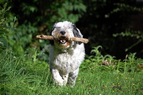
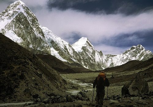
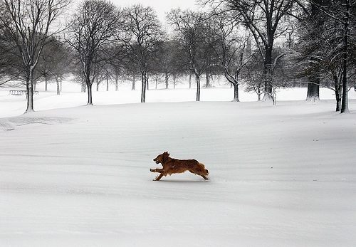
You can also play with the model. We hosted the Gradio app at Hugging Face!

Quick Recap

We’ve just explored the fascinating world of image captioning using the ResNet+LSTM architecture. Let’s summarize the key steps we covered:

• Understanding the Problem: Image captioning bridges computer vision and natural language processing, enabling a model to “see” an image and “describe” it in words.
• Applications: From accessibility tools for visually impaired users to enhancing SEO for e-commerce and powering robotic navigation systems, the potential use cases of image captioning are diverse and impactful.
• Architecture: The model is built on two pillars:
  • ResNet: Acts as the “eyes,” extracting high-level visual features from images using convolutional layers and residual connections.
  • LSTM: Serves as the “mouth,” decoding the extracted features into coherent textual descriptions by leveraging memory gates to handle sequential data.
• Training Pipeline:
  • Built a vocabulary to map words to indices.
  • Used the Flickr8k dataset to pair images with captions.
  • Trained the ResNet encoder and LSTM decoder jointly to minimize the difference between predicted and ground-truth captions.
• Inference: Generated captions for unseen images using the trained model, leveraging transformations, ResNet features, and LSTM-based decoding.
• Gradio Interface: Provided an interactive UI for users to upload images and get captions, making the model accessible for real-world use.

Conclusion

Image captioning isn’t just about teaching machines to “see and speak”- it’s about giving them the ability to tell stories, much like how “we” humans describe what we experience. The ResNet+LSTM pipeline we explored is a fantastic starting point: straightforward, effective, and packed with learning opportunities. From powering e-commerce searches to making the web accessible for all, its potential is both practical and exciting. Sure, the world is buzzing with transformers, but classics like this remind us that simplicity often packs magic. So, play with the code, run some images through it, and let your model spell some cool captions. If you get a good one, let us know in the comments!

See you soon, Happy New Year 😄

References

He, Kaiming, et al. “Deep residual learning for image recognition.” Proceedings of the IEEE conference on computer vision and pattern recognition. 2016.

Sepp Hochreiter, Jurgen Schmidhuber, “Long Short-Term Memory.”

Illustrated Guide to LSTM’s and GRU’s: A step by step explanation

How ResNet works, a GIF animation/illustration. No Code.