You can either love YOLOv5 or despise it. You can’t ignore YOLOv5!
YOLOv5 has gained much traction, controversy, and appraisals since its first release in 2020. Recently, YOLOv5 extended support to the OpenCV DNN framework, which added the advantage of using this state-of-the-art object detection model – Yolov5 OpenCV DNN Module.
We have been experimenting with YOLOv5 for a while, and it has a lot of ongoing interesting things. We are articulating our findings which include the following.
| ✅ Yolov5 inference using Ultralytics Repo and PyTorchHub ✅ Convert a YOLOv5 PyTorch model to ONNX ✅ Object detection using YOLOv5 and OpenCV DNN module. |
- Why use OpenCV for Deep Learning Inference?
- Why YOLOv5?
- A brief overview of YOLOv5
- Object Detection using YOLOv5 using OpenCV DNN (C++ and Python)
- Inference with YOLOv5
- Results and YOLOv5 Models Comparisons
YOLO Master Post – Every Model Explained
Don’t miss out on this comprehensive resource — Mastering All Yolo Models for a richer, more informed perspective on the YOLO series.
Why Use OpenCV for Deep Learning Inference?
The availability of a DNN model in OpenCV makes it super easy to perform Inference. Imagine you have an old object detection model in production, and you want to use this new state-of-the-art model instead. You may have to install multiple libraries to get it working.
Moreover, your production environment might not allow you to update software at will. This is where the OpenCV DNN module shines, as it has a single API for performing Deep Learning inference and has very few dependencies.
If you use OpenCV DNN, you may be able to swap out your old model for the latest one with very few changes to your production code.
Secondly, if you want to deploy a Deep Learning model in C++, it becomes a hassle, but it’s effortless to deploy in C++ using OpenCV.
Finally, OpenCV CPU implementation is highly optimized for Intel processors so that might be another reason to consider OpenCV DNN for inference.
Why YOLOv5?
YOLOv5 is fast and easy to use. It is based on the PyTorch framework, which has a larger community than Yolo v4 Darknet. The installation is simple and straightforward. Unlike YOLOv4, you don’t have to struggle to build it from the source, not even with CUDA support.
You can choose from ten available multi-scale models having speed/accuracy tradeoffs. It supports 11 different formats (both export and run time). Due to the advantages of Python-based core, it can be easily implemented in EDGE devices.
iDetect is an iOS app owned by Ultralytics, the company that developed YOLOv5. It can perform real-time object detection on phones using YOLOv5. Let us go through a brief history of YOLO before plunging into the code.
A Brief Overview of YOLOv5
The name YOLOv5 does tend to confuse the CV community, given that it is not exactly the updated version of YOLOv4. In fact, three major versions of YOLO were released in a short period in 2020.
- April: YOLOv4 by Alexey Bochkovskiy et al.
- June: YOLOv5 by Glenn Joscher, Ultralytics. GitHub
- July: PP-YOLO by Xiang Long et al.
Although they are based on YOLOv3, all are independent development. You can also check out our previous article on YOLOv3. The architecture of a Fully Connected Neural Network comprises the following.
- Backbone: The model backbone primarily extracts the essential features of an image.
- Head: The head contains the output layers that have final detections.
- Neck: The neck connects the backbone and the head. It mostly creates feature pyramids. The role of the neck is to collect feature maps of different stages.

Fig: YOLO architecture overview
As of now (12th April 2022), two years since the initial release, YOLOv5 still has not published a paper. Therefore, we don’t have detailed information on the architecture yet. The info provided in this article is from the GitHub readme, issues, release notes, and .yaml configuration files. However, it is in a very active development state, and we can expect further improvements with time. The following table summarizes the architecture of v3, v4, and v5.

Table: Model architecture summary, YOLO v3, v4 and v5
YOLOv4 is the official successor of YOLOv3 as it has been forked from the main repository pjredii/darknet. Written in C++, the framework is Darknet. YOLOv5, on the other hand, is different from previous releases. It is based on the Pytorch framework. The major improvements in YOLOv5 are,
- Mosaic Data Augmentation
- Auto Learning Bounding Box Anchors
Initially, YOLOv5 did not have substantial improvements over YOLOv4. However, recent releases have proved to be better in many areas. A recent paper on YOLO (July 2021), YOLOX: Exceeding YOLO Series in 2021, reports the superiority of YOLOv5 over YOLOv4 in terms of speed and accuracy. However, according to the report, not all YOLOv5 models could beat YOLOv4.
A detailed comparison of YOLOv5, YOLOv6, and YOLOv7 provides an invaluable resource in this regard. This comprehensive analysis dives deep into each model’s specifics, covering all these important aspects to help you get answers and decide.

Table: Comparison of the speed and accuracy of different object detectors on COCO 2017 test-dev. Source.
YOLOv5 was released with four models at first. Small, Medium, Large, and Extra large. Recently, YOLOv5 Nano and support for OpenCV DNN were introduced. Currently, each model has two versions, P5 and P6.
- P5: Three output layers, P3, P4, and P5. Trained on 640×640 images.
- P6: Four output layers, P3, P4, P5, and P6. Trained on 1280×1280 images.
| Models | Nano | Small | Medium | Large | Extra-Large |
| P5 | YOLOv5n | YOLOv5s | YOLOv5m | YOLOv5l | YOLOv5x |
| P6 | YOLOv5n6 | YOLOv5s6 | YOLOv5m6 | YOLOv5l6 | YOLOv5x6 |
Table: List of YOLOv5 P5 and P6 models
So it has a total of 10 compound-scaled object detection models. We will see more about their performance later but first, let us see how to perform object detection using OpenCV DNN and YOLOv5.
Object Detection using YOLOv5 and OpenCV DNN(C++ and Python)
4.1 CODE DOWNLOAD
The downloadable code folder contains Python and C++ scripts and a colab notebook. Go ahead and install the dependencies using the following command.
pip install -r requirements.txt
4.2 YOLOv5 MODEL CONVERSION
As the native platform of YOLOv5 is PyTorch, the models are available in .pt format. However, OpenCV DNN supports models in .onnx format. Therefore, we need to perform the model conversion. Follow the steps below to convert models to the required format.
- Clone the repository
- Install the requirements
- Download the PyTorch models
- Export to ONNX
NOTE: Nano, small, and medium ONNX models are included in the code folder.
It is possible to perform the conversion locally, but we recommend using colab to avoid getting stuck in resolving dependencies and downloading huge chunks of data. The following commands are for converting the YOLOv5s model. The notebook contains the code to convert and download the rest of the models.
# Clone the repository.
!git clone https://github.com/ultralytics/YOLOv5

%cd YOLOv5 # Install dependencies.
!pip install -r requirements.txt
!pip install onnx

# Download .pt model.
!wget https://github.com/ultralytics/YOLOv5/releases/download/v6.1/YOLOv5s.pt

%cd .. # Export to ONNX.
!python export.py --weights models/YOLOv5s.pt --include onnx

# Download the file.
from google.colab import files
files.download('models/YOLOv5s.onnx')
4.3 CODE EXPLANATION | YOLOv5 OpenCV DNN
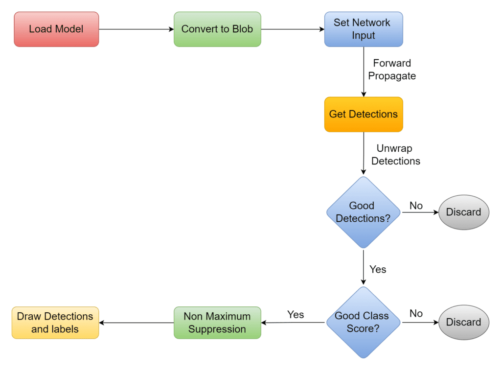
Now that we have the requirements ready, it’s time to start with the code. The following chart demonstrates the YOLOv5 with OpenCV DNN workflow.
4.3.1 Import Libraries
C++
#include <opencv2/opencv.hpp>
#include <fstream>
// Namespaces.
using namespace cv;
using namespace std;
using namespace cv::dnn;
Python
import cv2
import numpy as np
4.3.2 Define Global Parameters
The constants INPUT_WIDTH and INPUT_HEIGHT are for the blob size. The BLOB stands for Binary Large Object. It contains the data in readable raw format. The image must be converted to a blob so the network can process it. In our case, it is a 4D array object with the shape (1, 3, 640, 640).
SCORE_THRESHOLD: To filter low probability class scores.NMS_THRESHOLD: To remove overlapping bounding boxes.CONFIDENCE_THRESHOLD: Filters low probability detections.
We will discuss more of these parameters while going through the code.
Note: Unlike C++ the input size values in Python can not be of float type.
C++
// Constants.
const float INPUT_WIDTH = 640.0;
const float INPUT_HEIGHT = 640.0;
const float SCORE_THRESHOLD = 0.5;
const float NMS_THRESHOLD = 0.45;
const float CONFIDENCE_THRESHOLD = 0.45;

// Text parameters.
const float FONT_SCALE = 0.7;
const int FONT_FACE = FONT_HERSHEY_SIMPLEX;
const int THICKNESS = 1;

// Colors.
Scalar BLACK = Scalar(0,0,0);
Scalar BLUE = Scalar(255, 178, 50);
Scalar YELLOW = Scalar(0, 255, 255);
Scalar RED = Scalar(0,0,255);
Python
# Constants.
INPUT_WIDTH = 640
INPUT_HEIGHT = 640
SCORE_THRESHOLD = 0.5
NMS_THRESHOLD = 0.45
CONFIDENCE_THRESHOLD = 0.45

# Text parameters.
FONT_FACE = cv2.FONT_HERSHEY_SIMPLEX
FONT_SCALE = 0.7
THICKNESS = 1

# Colors.
BLACK  = (0,0,0)
BLUE   = (255,178,50)
YELLOW = (0,255,255)
4.3.3 Draw YOLOv5 Inference Label
The function draw_label annotates the class names anchored to the top left corner of the bounding box. The code is fairly simple. We pass the text string as a label in the argument, which is passed to the OpenCV function getTextSize().
It returns the bounding box size that the text string would take up. These dimension values are used to draw a black background rectangle on which the label is rendered by putText() function.
C++
void draw_label(Mat& input_image, string label, int left, int top)
{
    // Display the label at the top of the bounding box.
    int baseLine;
    Size label_size = getTextSize(label, FONT_FACE, FONT_SCALE, THICKNESS, &baseLine);
    top = max(top, label_size.height);
    // Top left corner.
    Point tlc = Point(left, top);
    // Bottom right corner.
    Point brc = Point(left + label_size.width, top + label_size.height + baseLine);
    // Draw white rectangle.
    rectangle(input_image, tlc, brc, BLACK, FILLED);
    // Put the label on the black rectangle.
    putText(input_image, label, Point(left, top + label_size.height), FONT_FACE, FONT_SCALE, YELLOW, THICKNESS);
}
Python
def draw_label(im, label, x, y):
    """Draw text onto image at location."""
    # Get text size.
    text_size = cv2.getTextSize(label, FONT_FACE, FONT_SCALE, THICKNESS)
    dim, baseline = text_size[0], text_size[1]
    # Use text size to create a BLACK rectangle.
    cv2.rectangle(im, (x,y), (x + dim[0], y + dim[1] + baseline), (0,0,0), cv2.FILLED);
    # Display text inside the rectangle.
    cv2.putText(im, label, (x, y + dim[1]), FONT_FACE, FONT_SCALE, YELLOW, THICKNESS, cv2.LINE_AA)
4.3.4 PRE-PROCESSING YOLOv5 Model
The function pre–process takes the image and the network as arguments. At first, the image is converted to a blob. Then it is set as input to the network. The function getUnconnectedOutLayerNames() provides the names of the output layers. It has features of all the layers, through which the image is forward propagated to acquire the detections. After processing, it returns the detection results.
C++
vector<Mat> pre_process(Mat &input_image, Net &net)
{
    // Convert to blob.
    Mat blob;
    blobFromImage(input_image, blob, 1./255., Size(INPUT_WIDTH, INPUT_HEIGHT), Scalar(), true, false);

    net.setInput(blob);

    // Forward propagate.
    vector<Mat> outputs;
    net.forward(outputs, net.getUnconnectedOutLayersNames());

    return outputs;
}
Python
def pre_process(input_image, net):
      # Create a 4D blob from a frame.
      blob = cv2.dnn.blobFromImage(input_image, 1/255,  (INPUT_WIDTH, INPUT_HEIGHT), [0,0,0], 1, crop=False)

      # Sets the input to the network.
      net.setInput(blob)

      # Run the forward pass to get output of the output layers.
      outputs = net.forward(net.getUnconnectedOutLayersNames())
      return outputs
4.3.5 POST-PROCESSING YOLOv5 Prediction Output
In the previous function pre_process, we get the detection results as an object. It needs to be unwrapped for further processing. Before discussing the code any further, let us see the shape of this object and what it contains.
The returned object is a 2-D array. The output depends on the size of the input. For example, with the default input size of 640, we get a 2D array of size 25200×85 (rows and columns). The rows represent the number of detections. So each time the network runs, it predicts 25200 bounding boxes. Every bounding box has a 1-D array of 85 entries that tells the quality of the detection. This information is enough to filter out the desired detections.

The first two places are normalized center coordinates of the detected bounding box. Then comes the normalized width and height. Index 4 has the confidence score that tells the probability of the detection being an object. The following 80 entries tell the class scores of 80 objects of the COCO dataset 2017, on which the model has been trained.
Fun Fact: The COCO dataset 2017 has a total of 91 objects. However, 11 objects are still missing labels.
A. Filter Good Detections given by YOLOv5 Models
While unwrapping, we need to be careful with the shape. With OpenCV-Python 4.5.5, the object is a tuple of a 3-D array of size 1x row x column. It should be row x column. Hence, the array is accessed from the zeroth index. This issue is not observed in the case of C++.
The network generates output coordinates based on the input size of the blob, i.e. 640. Therefore, the coordinates should be multiplied by the resizing factors to get the actual output. The following steps are involved in unwrapping the detections.
- Loop through detections.
- Filter out good detections.
- Get the index of the best class score.
- Discard detections with class scores lower than the threshold value.
C++
Mat post_process(Mat &input_image, vector<Mat> &outputs, const vector<string> &class_name)
{
    // Initialize vectors to hold respective outputs while unwrapping     detections.
    vector<int> class_ids;
    vector<float> confidences;
    vector<Rect> boxes;
    // Resizing factor.
    float x_factor = input_image.cols / INPUT_WIDTH;
    float y_factor = input_image.rows / INPUT_HEIGHT;
    float *data = (float *)outputs[0].data;
    const int dimensions = 85;
    // 25200 for default size 640.
    const int rows = 25200;
    // Iterate through 25200 detections.
    for (int i = 0; i < rows; ++i)
    {
        float confidence = data[4];
        // Discard bad detections and continue.
        if (confidence >= CONFIDENCE_THRESHOLD)
        {
            float * classes_scores = data + 5;
            // Create a 1x85 Mat and store class scores of 80 classes.
            Mat scores(1, class_name.size(), CV_32FC1, classes_scores);
            // Perform minMaxLoc and acquire the index of best class  score.
            Point class_id;
            double max_class_score;
            minMaxLoc(scores, 0, &max_class_score, 0, &class_id);
            // Continue if the class score is above the threshold.
            if (max_class_score > SCORE_THRESHOLD)
            {
                // Store class ID and confidence in the pre-defined respective vectors.
                confidences.push_back(confidence);
                class_ids.push_back(class_id.x);
                // Center.
                float cx = data[0];
                float cy = data[1];
                // Box dimension.
                float w = data[2];
                float h = data[3];
                // Bounding box coordinates.
                int left = int((cx - 0.5 * w) * x_factor);
                int top = int((cy - 0.5 * h) * y_factor);
                int width = int(w * x_factor);
                int height = int(h * y_factor);
                // Store good detections in the boxes vector.
                boxes.push_back(Rect(left, top, width, height));
            }
        }
        // Jump to the next row.
        data += 85;
    }
Python
def post_process(input_image, outputs):
      # Lists to hold respective values while unwrapping.
      class_ids = []
      confidences = []
      boxes = []
      # Rows.
      rows = outputs[0].shape[1]
      image_height, image_width = input_image.shape[:2]
      # Resizing factor.
      x_factor = image_width / INPUT_WIDTH
      y_factor =  image_height / INPUT_HEIGHT
      # Iterate through detections.
      for r in range(rows):
            row = outputs[0][0][r]
            confidence = row[4]
            # Discard bad detections and continue.
            if confidence >= CONFIDENCE_THRESHOLD:
                  classes_scores = row[5:]
                  # Get the index of max class score.
                  class_id = np.argmax(classes_scores)
                  #  Continue if the class score is above threshold.
                  if (classes_scores[class_id] > SCORE_THRESHOLD):
                        confidences.append(confidence)
                        class_ids.append(class_id)
                        cx, cy, w, h = row[0], row[1], row[2], row[3]
                        left = int((cx - w/2) * x_factor)
                        top = int((cy - h/2) * y_factor)
                        width = int(w * x_factor)
                        height = int(h * y_factor)
                        box = np.array([left, top, width, height])
                        boxes.append(box)
B. Remove Overlapping Boxes Predicted by YOLOv5
After filtering good detections, we are left with the desired bounding boxes. However, there can be multiple overlapping bounding boxes, which may look like the following.

This is solved by performing Non-Maximum Suppression. The function NMSBoxes() takes a list of boxes, calculates IOU (Intersection Over Union), and decides to keep the boxes depending on the NMS_THRESHOLD. Curious about how it works? Check out Non Maximum Suppression to know more.
C++
    // Perform Non-Maximum Suppression and draw predictions.
    vector<int> indices;
    NMSBoxes(boxes, confidences, SCORE_THRESHOLD, NMS_THRESHOLD, indices);
    for (int i = 0; i < indices.size(); i++)
    {
        int idx = indices[i];
        Rect box = boxes[idx];
        int left = box.x;
        int top = box.y;
        int width = box.width;
        int height = box.height;
        // Draw bounding box.
        rectangle(input_image, Point(left, top), Point(left + width, top + height), BLUE, 3*THICKNESS);
        // Get the label for the class name and its confidence.
        string label = format("%.2f", confidences[idx]);
        label = class_name[class_ids[idx]] + ":" + label;
        // Draw class labels.
        draw_label(input_image, label, left, top);
    }
    return input_image;
}
Python
 # Perform non maximum suppression to eliminate redundant, overlapping boxes with lower confidences.
      indices = cv2.dnn.NMSBoxes(boxes, confidences, CONFIDENCE_THRESHOLD, NMS_THRESHOLD)
      for i in indices:
            box = boxes[i]
            left = box[0]
            top = box[1]
            width = box[2]
            height = box[3]
            # Draw bounding box.
            cv2.rectangle(input_image, (left, top), (left + width, top + height), BLUE, 3*THICKNESS)
            # Class label.
            label = "{}:{:.2f}".format(classes[class_ids[i]], confidences[i])
            # Draw label.
            draw_label(input_image, label, left, top)
      return input_image
4.3.6 Main Function
Finally, we load the model. Perform pre-processing and post-processing followed by displaying efficiency information.
C++
int main()
{
    // Load class list.
    vector<string> class_list;
    ifstream ifs("coco.names");
    string line;
    while (getline(ifs, line))
    {
        class_list.push_back(line);
    }
    // Load image.
    Mat frame;
    frame = imread("traffic.jpg");
    // Load model.
    Net net;
    net = readNet("YOLOv5s.onnx");
    vector<Mat> detections;     // Process the image.
    detections = pre_process(frame, net);
    Mat img = post_process(frame.clone(), detections, class_list);
    // Put efficiency information.
    // The function getPerfProfile returns the overall time for     inference(t) and the timings for each of the layers(in layersTimes).
    vector<double> layersTimes;
    double freq = getTickFrequency() / 1000;
    double t = net.getPerfProfile(layersTimes) / freq;
    string label = format("Inference time : %.2f ms", t);
    putText(img, label, Point(20, 40), FONT_FACE, FONT_SCALE, RED);
    imshow("Output", img);
    waitKey(0);
    return 0;
}
Python
if __name__ == '__main__':
      # Load class names.
      classesFile = "coco.names"
      classes = None
      with open(classesFile, 'rt') as f:
            classes = f.read().rstrip('\n').split('\n')
      # Load image.
      frame = cv2.imread(‘traffic.jpg)
      # Give the weight files to the model and load the network using       them.
      modelWeights = "YOLOv5s.onnx"
      net = cv2.dnn.readNet(modelWeights)
      # Process image.
      detections = pre_process(frame, net)
      img = post_process(frame.copy(), detections)
      """
      Put efficiency information. The function getPerfProfile returns       the overall time for inference(t)
      and the timings for each of the layers(in layersTimes).
      """
      t, _ = net.getPerfProfile()
      label = 'Inference time: %.2f ms' % (t * 1000.0 /  cv2.getTickFrequency())
      print(label)
      cv2.putText(img, label, (20, 40), FONT_FACE, FONT_SCALE,  (0, 0, 255), THICKNESS, cv2.LINE_AA)
      cv2.imshow('Output', img)
      cv2.waitKey(0)
Inference with YOLOv5
Now that you know how to perform object detection using YOLOv5 and OpenCV let us also see how to do the same using the repository. Object detection using YOLOv5 is super simple. There are two ways to perform inference using the out-of-the-box code.
- Ultralytics Repository
- PyTorchHub
The basic guideline is already provided in the GitHub readme. Here, we will walk through a little more detail on what else can be done. Let us go ahead and clone the GitHub repository using the command below.
git clone https://github.com/ultralytics/yolov5.git
5.1 Using the YOLOv5 Ultralytics Repository
The script detect.py is in the root directory of the YOLOv5 repository. We can run it as a normal python script. The only necessary argument is the source path. The models are downloaded from the latest YOLOv5 release. It saves the results to ./yolov5/runs/detect. As mentioned in the GitHub readme, the following sources can be used.
| Input Source | Description |
| Webcam | Can be accessed using 0, 1, 2, and so on; depending on the number of connected webcams. |
| Image | Although the official readme says .jpg, you can use many more image formats. We have tested most of them and it works fine. Currently jpeg, png, tif, tiff, dng, webp and mpo are supported. |
| Video | Similarly, for videos too, it’s not only .mp4 but also mov, avi, mpg, mpeg, m4v, wmv and mkv. |
| Path | We can also provide the path of a directory containing different images and videos. It will process all the supported files one by one. If required, you can also specify the type of file, i.e., path/*.mp4. |
| YouTube link | A super useful feature to process YouTube videos directly. However, to make it work, we need youtube-dl and pafy to be installed. You can install them using the following command.pip install youtube_dl pafy |
| RTSP, RTMP and HTTP stream | YouTube live stream works well, given that youtube-dl and pafy are installed. But we could not make RTSP stream work using this sample bunny video stream. Neither did Facebook live streams. The source code seems to be supporting YouTube live links as of now. |
YOLOv5 inference with default settings generates a log that looks something like the following. Let us go through some of the inference attributes.
detect: weights=yolov5s.pt, source=C:\Users\Kukil\Desktop\image.jpg, data=data\coco128.yaml, imgsz=[640, 640], conf_thres=0.25, iou_thres=0.45, max_det=1000, device=, view_img=False, save_txt=False, save_conf=False, save_crop=False, nosave=False, classes=None, agnostic_nms=False, augment=False, visualize=False, update=False, project=runs\detect, name=exp, exist_ok=False, line_thickness=3, hide_labels=False, hide_conf=False, half=False, dnn=False
YOLOv5  v6.1-124-g8c420c4 torch 1.11.0+cpu CPU
| Flags | Description |
| Weights | using the --weights flag followed by the model name. At first, the program looks for the model in the root directory and downloads it if not available. Note that we can use any format from the list of 11 supported platforms. |
| Input size | A factor that hugely impacts the speed and accuracy of a model. The flag is --imgsz x y , where x and y are blob input size. |
| Confidence threshold | By default, the confidence threshold is 0.25. Use the flag --conf_thresh to change the threshold. |
| IOU threshold | IOU stands for Intersection Over Union. This threshold is for performing Non-maximum suppression. Try playing with the default value 0.45 to see how it impacts the results. Flag --iou_thresh. |
| DNN | Using the flag –dnn lets the program use OpenCV DNN for ONNX inference. |
5.2 Using PyTorchHub to run YOLOv5 Inference
The following script downloads a pre-trained model from PyTorchHub and passes an image for inference. By default, yolov5s.pt is downloaded unless the name is changed. The results can be printed to the console, saved to ./yolov5/runs/hub, displayed on the screen(local), and returned as tensors or pandas data frames. You can also play with various inference attributes.
import cv2
import torch
# Model
model = torch.hub.load('ultralytics/yolov5', 'yolov5s')
# Image
img = cv2.imread(PATH_TO_IMAGE)
# Inference
results = model(imgs, size=640)  # includes NMS
# Results
results.print()
results.save()
Although both Ultralytics Repository and PyTorchHub methods are decent, they have limited functionalities. We could edit the source code, but a better way is to write it from scratch. That way, we get better control over the code, with the advantage of coding in C++.
Results and Comparisons of YOLOv5 Models
6.1 YOLOv5 Nano vs Medium vs Extra-Large
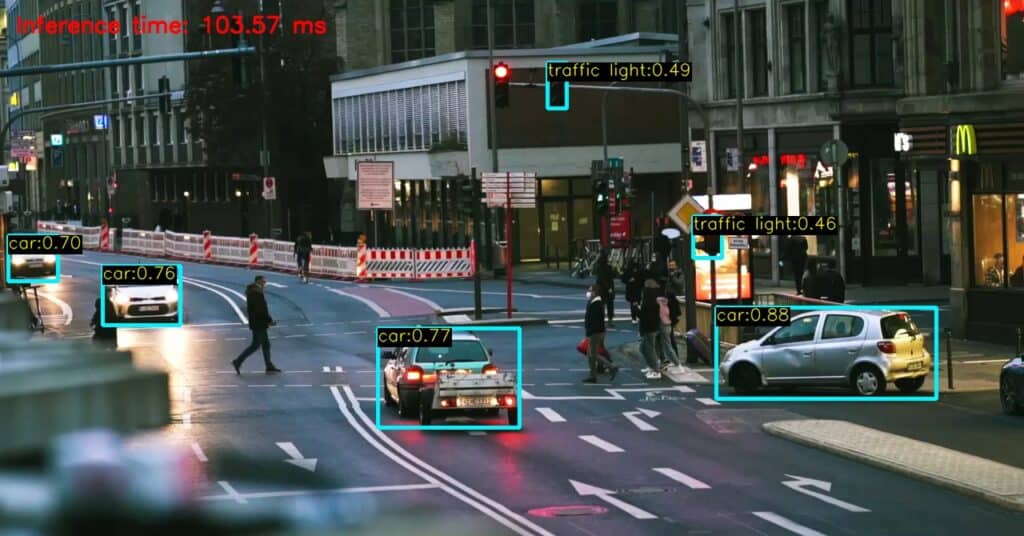
The following two results have been obtained using the nano, medium, and extra-large models. In terms of accuracy, the extra-large model dominates. It can even detect objects that our eyes can miss. On the other hand, nano is about 10x faster but less accurate.
# Test environment configurations.
CPU: AMD RYZEN 5 4600
Input size = 640
Batch size = 1
Fig: Results obtained using the YOLOv5n model
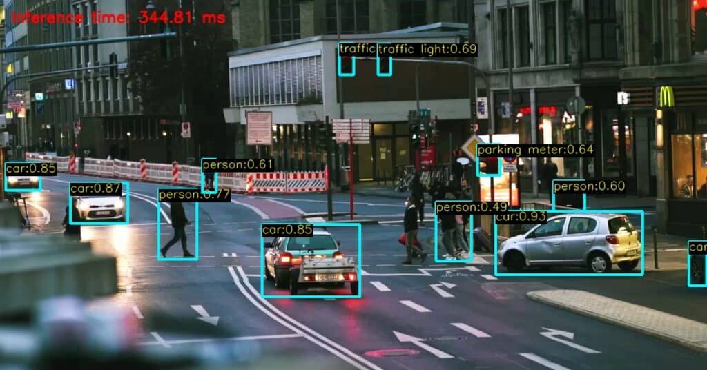
Fig: Result obtained using YOLOv5m model
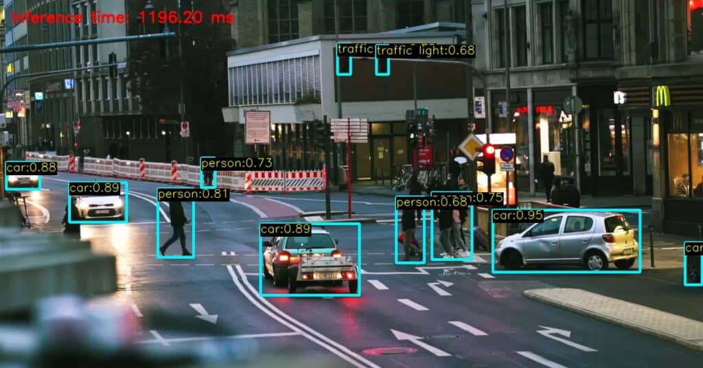
Fig: Results obtained using the YOLOv5x model
6.2 YOLOv5 Speed test with input size variations | Yolov5 OpenCV
In this speed test, we are taking the same image but varying blob sizes. Time(ms) is measured by running the inference 20 times per image and then taking the average. The same experiment is repeated for nano, small and medium models, and the following results have been obtained.
Note: To run an inference with different input sizes, models must be exported accordingly. For example, to set 480 as the input size, export the model using the following command. This is done to optimize ONNX models as they are meant for deployment.
!python export.py --weights models/YOLOv5s.pt --include onnx -imsz 480 480
However, we don’t have to convert all the models for performing tests. Use the flag —dynamic while exporting to obtain the dynamic model. No need to mention specific input size. Then we can perform inference in ONNX runtime using the Ultralytics Repository as shown below. Where size is a multiple of 32.
python detect.py --source image.jpg --weights yolov5n-dynamic.onnx --imgsz size size

Table: Speed test by varying the input size
We can see great improvement in speed but at the cost of accuracy. Following are the results obtained on varying input sizes to YOLOv5 medium.

Fig: Inference using YOLOv5m, size = 640

Fig: Inference using YOLOv5m, size = 480

Fig: Inference using YOLOv5m, size = 320
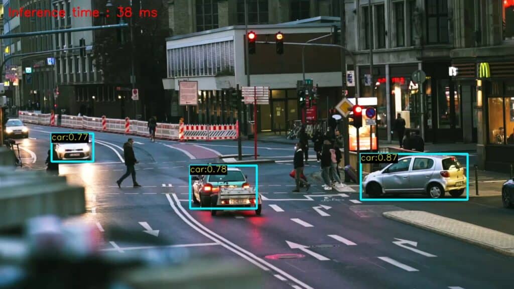
Fig: Inference using YOLOv5m, size = 160
6.3 Speed analysis of YOLOv5 Models
The following chart shows a comparison of different YOLOv5 model speeds. Results might vary from device to device, but we get an overall idea of the speed vs. accuracy tradeoff. You can decide to choose a model depending on your requirement.
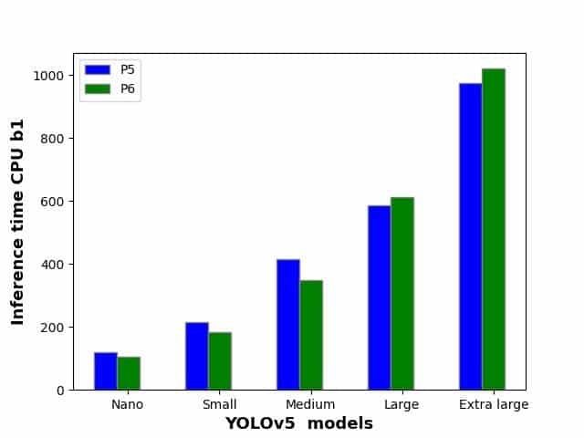
Fig: Inference time by YOLOv5 P5 and P6 models.
CONCLUSION
In this post, we discussed inference using out-of-the-box code in detail and using the YOLOv5 model in OpenCV with C++ and Python. You also learned how to convert a PyTorch model to ONNX format.
Dive deeper into personalized model training with YOLOv5 – Custom Object Detection Training, a guide focused on tailoring YOLOv5 for specific detection tasks.
Further explore YOLOv5’s capabilities in our guide ‘Getting Started with YOLOv5 Instance Segmentation, perfect for those looking to delve into advanced segmentation techniques.
I hope you enjoyed reading the article. Have any questions or suggestions? Add your comments below.


