


What is YOLOv7?
YOLOv7 is a single-stage real-time object detector. It was introduced to the YOLO family in July’22. According to the YOLOv7 paper, it is the fastest and most accurate real-time object detector to date. YOLOv7 established a significant benchmark by taking its performance up a notch.
This article contains simplified YOLOv7 paper explanation and inference tests. We will go through the YOLOv7 GitHub repository and test inference. We will also see how YOLOv7 compares with other object detectors of the YOLO family.
| What will be covered in the post? 1. YOLOv7 architecture, What’s new? 2. Object Detection using YOLOv7 3. YOLOv7 models and comparative analysis 4. YOLOv7 Pose: Human Pose Estimation |
- YOLO Architecture in General
- What’s new in YOLOv7?
- YOLOv7 Architecture
- Trainable Bag of Freebies in YOLOv7
- YOLOv7 Experiments and Results
- YOLOv7 Object Detection Inference
- Comparison between YOLOv4, YOLOv5-Large and YOLOv7
- YOLOv7 Pose Estimation
- Summary of YOLOv7
YOLO Master Post – Every Model Explained
Don’t miss out on this comprehensive resource, Mastering All Yolo Models for a richer, more informed perspective on the YOLO series.
YOLO Architecture in General
YOLO architecture is FCNN(Fully Connected Neural Network) based. However, Transformer-based versions have also recently been added to the YOLO family. We will discuss Transformer based detectors in a separate post. For now, let’s focus on FCNN (Fully Convolutional Neural Network) based YOLO object detectors.
The YOLO framework has three main components.
- Backbone
- Head
- Neck
The Backbone mainly extracts essential features of an image and feeds them to the Head through Neck. The Neck collects feature maps extracted by the Backbone and creates feature pyramids. Finally, the head consists of output layers that have final detections. The following table shows the architectures of YOLOv4, YOLOv4, and YOLOv5.
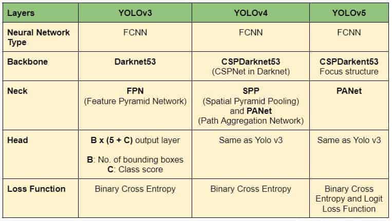
Table1: Model architecture summary of YOLOv3, YOLOv4, and YOLOv5
Apart from architectural modifications, there are several other improvements. Go through the YOLO series for detailed information.


What’s New in YOLOv7?
YOLOv7 improves speed and accuracy by introducing several architectural reforms. Similar to Scaled YOLOv4, YOLOv7 backbones do not use ImageNet pre-trained backbones. Rather, the models are trained using the COCO dataset entirely. The similarity can be expected because YOLOv7 is written by the same authors as Scaled YOLOv4, which is an extension of YOLOv4. The following major changes have been introduced in the YOLOv7 paper. We will go through them one by one.
- Architectural Reforms
- E-ELAN (Extended Efficient Layer Aggregation Network)
- Model Scaling for Concatenation-based Models
- Trainable BoF (Bag of Freebies)
- Planned re-parameterized convolution
- Coarse for auxiliary and Fine for lead loss
YOLOv7 Architecture
The architecture is derived from YOLOv4, Scaled YOLOv4, and YOLO-R. Using these models as a base, further experiments were carried out to develop new and improved YOLOv7.
E-ELAN (Extended Efficient Layer Aggregation Network) in YOLOv7 paper
The E-ELAN is the computational block in the YOLOv7 backbone. It takes inspiration from previous research on network efficiency. It has been designed by analyzing the following factors that impact speed and accuracy.
- Memory access cost
- I/O channel ratio
- Element wise operation
- Activations
- Gradient path
| The proposed E-ELAN uses expand, shuffle, and merge cardinality to achieve the ability to continuously enhance the learning ability of the network without destroying the original gradient path. |
In simple terms, E-ELAN architecture enables the framework to learn better. It is based on the ELAN computational block. The ELAN paper has not been published yet when writing this post. We will update the post by adding ELAN details when available.

Fig: E-ELAN and previous work on maximal layer efficiency
Compound Model Scaling in YOLOv7
Different applications require different models. While some need highly accurate models, some prioritize speed. Model scaling is performed to suit these requirements and make it fit in various computing devices.
While scaling a model size, the following parameters are considered.
- Resolution ( size of the input image)
- Width (number of channels)
- Depth (number of layers)
- Stage (number of feature pyramids)
NAS (Network Architecture Search) is a commonly used model scaling method. It is used by researchers to iterate through the parameters to find the best scaling factors. However, methods like NAS do parameter-specific scaling. The scaling factors are independent in this case.
The authors of the YOLOv7 paper show that it can be further optimized with a compound model scaling approach. Here, width and depth are scaled in coherence for concatenation-based models.
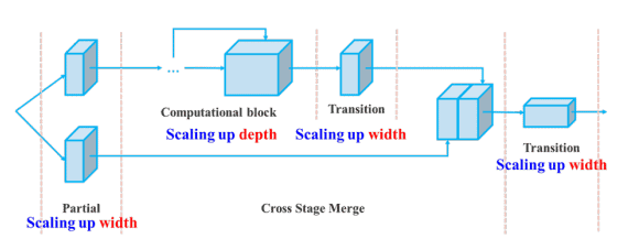
Fig: YOLOv7 compound scaling
Trainable Bag of Freebies in YOLOv7
BoF or Bag of Freebies are methods that increase the performance of a model without increasing the training cost. YOLOv7 has introduced the following BoF methods.
Planned Re-parameterized Convolution
Re-parameterization is a technique used after training to improve the model. It increases the training time but improves the inference results. Two types of re-parametrization are used to finalize models: Model level and Module level ensemble.
Model level re-parametrization can be done in the following two ways.
- Using different training data but the same settings, train multiple models. Then average their weights to obtain the final model.
- Take the average of the weights of models at different epochs.
Recently, Module level re-parameterization has gained a lot of traction in research. In this method, the model training process is split into multiple modules. The outputs are ensembled to obtain the final model. The authors in the YOLOv7 paper show the best possible ways to perform module-level ensemble (shown below).
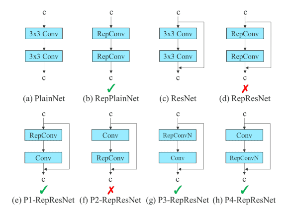
Fig: Re-parameterization trials
In the diagram above, The 3×3 convolution layer of the E-ELAN computational block is replaced with the RepConv layer. Experiments we carried out by switching or replacing the positions of RepConv, 3×3 Conv, and Identity connection. The residual bypass arrow shown above is an identity connection. It is nothing but a 1×1 convolutional layer. We can see the configurations that work and the ones that do not. Check out more about RepConv in the RepVGG paper.
Including RepConv, YOLOv7 also performs re-parameterization on Conv-BN (Convolution Batch Normalization), OREPA(Online Convolutional Re-parameterization), and YOLO-R to get the best results. We will discuss the implementation part in a separate post.
Coarse for Auxiliary and Fine for Lead Loss
As you already know by now, YOLO architecture comprises a backbone, a neck, and a head. The head contains the predicted outputs. YOLOv7 does not limit itself to a single head. It has multiple heads to do whatever it wants. Interesting, isn’t it?
However, it’s not the first time a multi-headed framework was introduced. Deep Supervision, a technique used by DL models, uses multiple heads. In YOLOv7, the head responsible for final output is called the Lead Head. And the head used to assist training in the middle layers is called the Auxiliary Head.
With the help of an assistant loss, the weights of the auxiliary heads are updated. It allows for Deep Supervision, and the model learns better. These concepts are closely coupled with the Lead Head and the Label Assigner.
Label Assigner is a mechanism that considers the network prediction results together with the ground truth and then assigns soft labels. It’s important to note that the label assigner generates soft and coarse labels instead of hard ones.
Lead Head Guided Label Assigner and Coarse-to-Fine Lead Head Guided Label Assigner
The Lead Head Guided Label Assigner encapsulates the following three concepts.
- Lead Head
- Auxiliary Head
- Soft Label Assigner
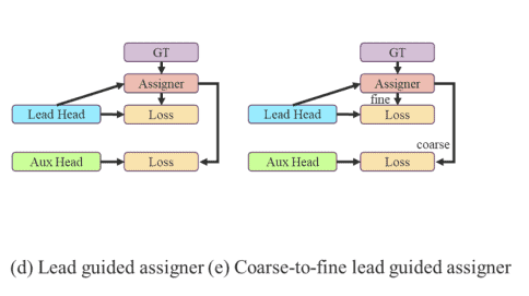
The Lead Head in the YOLOv7 network predicts the final results. Soft labels are generated based on these final results. The important part is that the loss is calculated for both the lead head and the auxiliary head based on the same soft labels that are generated. Ultimately, both heads get trained using the soft labels. This is shown in the left image in the above figure.
One may ask here, “why soft labels?”. The authors have put it quite well in the paper:
“The reason to do this is that the lead head has a relatively strong learning capability. So the soft label generated from it should be more representative of the distribution and correlation between the source data and the target. By letting the shallower auxiliary head directly learn the information that the lead head has learned, the lead head will be more able to focus on learning residual information that has not yet been learned.”
Now, coming to the coarse-to-fine labels as shown in the right image in the previous figure. In the above process, two sets of soft labels are generated.
- A fine label to train the lead head
- A set of coarse labels to train the auxiliary head.
The fine labels are the same as the directly generated soft labels. However, more grids are treated as positive targets to generate the coarse labels. This is done by relaxing the constraints of the positive sample assignment process.
YOLOv7 Experiments and Results
All the YOLOv7 models surpass the previous object detectors in speed and accuracy in the range of 5 FPS to 160 FPS. The following figure gives a pretty good idea about the Average Precision(AP) and speed of the YOLOv7 models compared to the others.
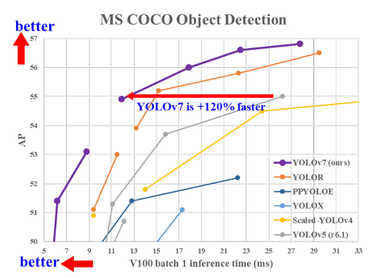
It is clear from the figure that starting from YOLOv7, there is no competition with YOLOv7 in terms of speed and accuracy.
Note: The results discussed further are from the YOLOv7 paper, where all the inference experiments were done on a Tesla V100 GPU. All AP results were done either on the COCO validation or test set.
mAP Comparison: YOLOv7 vs Others
The following table shows the comparison of YOLOv7 models with other baseline object detectors.

Table: YOLOv7 vs Other Baseline Models
The results shown above are mostly grouped together according to a range of parameters for a particular set of models.
- Starting with the YOLOv7-Tiny model, the smallest in the family with just over 6 million parameters. With a validation AP of 35.2%, it beats YOLOv4-Tiny models with similar parameters.
- The YOLOv7 normal model with almost 37 million parameters gives 51.2% AP. It beats variants of YOLOv4 and YOLOR, which have more parameters easily.
- The larger models in the YOLO7 family are YOLOv7-X, YOLOv7-E6, YOLOv7-D6, and YOLOv7-E6E. All of these beat the respective YOLOR models having either a similar or lesser number of parameters and giving APs of 52.9%, 55.9%, 56.3%, and 56.8%, respectively.
Now, it is not only the YOLOv4 and YOLOR models that YOLOv7 surpasses. Comparing the validation APs with that of the YOLOv5 and YOLOv7 models, which have parameters in the same range, it is pretty clear that YOLOv7 also beats all of the YOLOv5 models.
FPS Comparison: YOLOv7 vs Others
Table 2 in the YOLOv7 paper provides a comprehensive comparison of the FPS of YOLOv7 with other models. It also includes the COCO mAP comparison.
It is already established that the YOLOv7 has the highest FPS and mAP in the range of 5 FPS to 160 FPS. All the FPS comparisons were done on the Tesla V100 GPU.
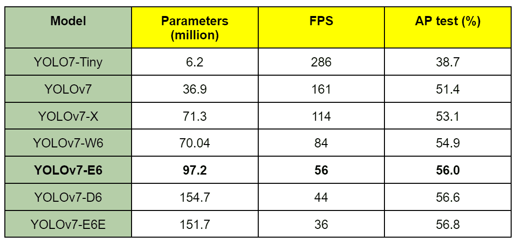
Table: YOLOv7 models FPS comparison
It is worth noting that none of the YOLOv7 models are meant for mobile devices/mobile CPUs (as mentioned in the YOLOv7 paper).
- YOLOv7-Tiny, YOLOv7, and YOLOv7-W6 are meant for edge GPU, normal (consumer) GPU, and cloud GPU, respectively.
- YOLOv7-E6 and YOLOv7-D6, and YOLOv7-E6E are also meant for high-end cloud GPUs only.
Nonetheless, all of the YOLOv7 models run at more than 30 FPS on the Tesla V100 GPU, which is more than real-time FPS.
The experiments above prove that YOLOv7 models outperform the existing object detectors. Both in terms of speed and accuracy.
???????? Skip to Training YOLOv7: Training YOLOv7 on Custom Pothole Dataset

YOLOv7 Object Detection Inference
Now, let’s get into the exciting part of the blog post, that is, running inference on videos using YOLOv7. We will run the inference using the YOLOv7 and YOLOv7-Tiny models. Along with that, we will also compare the results with that of the YOLOv5 and YOLOv4 models.
| Note: All the inference results shown here were run on a machine with 6 GB GTX 1060 (laptop GPU), 8th generation i7 CPU, and 16 GB of RAM. |
If you intend to run object detection inference experiments on your own videos, you have to clone the YOLOv7 GitHub repository using the following command.
git clone https://github.com/WongKinYiu/yolov7.git
Then you can use the detect.py script to run inference on the videos of your choice. You will also need to download the yolov7-tiny.pt and yolov7.pt pre-trained model.
Here, we will run inference on three videos depicting the following three different scenarios.
- The first video is to test how the YOLOv7 object detection models perform on small and far-off objects.
- The second video has a lot of people depicting a crowded scenario.
- And the third video is one where many YOLO models (v4, v5, and v7) make the same general mistake while detecting the objects.
The YOLOv7 results here are shown together for the Tiny and Normal models for all three videos. This will help us compare the results for each of the results in an easy manner.
Let’s check the detection inference results on the first video using the YOLOv7-Tiny (top) and YOLOv7 (bottom) models. The following commands were used to run the inference using the Tiny and Normal models.
python detect.py --source ../inference_data/video_1.mp4 --weights yolov7-tiny.pt --name video_tiny_1 --view-img
python detect.py --source ../inference_data/video_1.mp4 --weights yolov7.pt --name video_1 --view-img
YOLOv7-tiny
YOLOv7-Normal
We can see the limitations of the YOLOv7-Tiny model right away. It cannot detect cars, motorcycles, and persons who are very far off and small. The YOLOv7 model can detect these objects better. But that’s not the entire story. Although YOLO7-Tiny is not performing that well, it is much faster than YOLOv7. While YOLOv7 gave around 19 FPS, YOLOv7-Tiny ran it at around 42 FPS, which is well above real-time.
Now, let’s check out the results of the second video, which depicts a crowded scenario. We use the same command as above but change the values for the –source and –name flags depending on the video path and name.
YOLOv7 tiny
YOLOv7 Normal
The YOLOv7 model can detect persons with less fluctuation and more confidence compared to the YOLOv7-Tiny model. Not only that, but YOLOv7-Tiny is also missing out on some of the traffic lights and people who are far away.
Let’s run the inference on a final video that shows some general failure cases across all the YOLOv7 models.
YOLOv7 tiny
YOLOv7 Normal
We can see some of the general mistakes across both models:
- Detecting other road signs as stop signs.
- Detecting the forbidden road symbols as persons wrongly.
As we will see later, the above two mistakes are common across YOLOv4 and YOLOv5.
Even though the YOLO7-Tiny makes more mistakes than the YOLOv7 model, it is much faster. On average, the YOLOv7-Tiny runs at more than 40 FPS, while the YOLOv7 model runs at slightly above 20 FPS.
Comparison Between YOLOv4, YOLOv5-Large, and YOLOv7 Model
The following three videos show the comparison between the YOLOv4, YOLOv5-Large, and the YOLOv7 model (top to bottom) on one of the videos. This will give us a proper qualitative idea of how each model performs across various scenarios.
YOLOv4
YOLOv5-Large
YOLOv7
And the following table shows the FPS and run times for different variants of the three models on the three videos.

Table: YOLOv7 vs Other detectors inference speed chart
YOLOv7 Pose Estimation
YOLOv7 is the first in the YOLO family to include a human pose estimation model. This is really interesting because there are very few real-time models out there.
Recently, the official repository also got updated with a pre-trained pose estimation model. Hence, we will not cover the details in this post. A dedicated article on the internals of the YOLOv7 Pose Estimation model will be published later. In this section, we will discuss the application part and observe how it works.
| [Update: 18/10/22]: We have kept our promise. Check out the detailed YOLOv7 Pose Estimation article here. |
YOLOv7 Pose Prerequisites
First, please ensure that you have cloned the YOLOv7 GitHub repository. Now, execute the following command within the cloned yolov7 directory to download the pre-trained pose estimation model.
wget https://github.com/WongKinYiu/yolov7/releases/download/v0.1/yolov7-w6-pose.pt
YOLOv7 Pose Code
We will need a custom script to run pose estimation inference using the pre-trained model. Let’s write the code in a new yolov7_keypoint.py script inside the yolov7 directory.
import matplotlib.pyplot as plt
import torch
import cv2
import numpy as np
import time

from torchvision import transforms
from utils.datasets import letterbox
from utils.general import non_max_suppression_kpt
from utils.plots import output_to_keypoint, plot_skeleton_kpts

device = torch.device("cuda:0" if torch.cuda.is_available() else "cpu")
weigths = torch.load('yolov7-w6-pose.pt')
model = weigths['model']
model = model.half().to(device)
_ = model.eval()

video_path = '../inference_data/video_4.mp4'
We import all the required modules and load the pre-trained yolov7-w6-pose.pt model, and initialize a video_path variable for the path to the source video. If you intend to run this inference on your own videos, please change the video_path accordingly.
Next, let’s read the video from the disk and create the VideoWriter object to save the resulting video on the disk.
cap = cv2.VideoCapture(video_path)
if (cap.isOpened() == False):
  print('Error while trying to read video. Please check path again')

# Get the frame width and height.
frame_width = int(cap.get(3))
frame_height = int(cap.get(4))

# Pass the first frame through `letterbox` function to get the resized image,
# to be used for `VideoWriter` dimensions. Resize by larger side.
vid_write_image = letterbox(cap.read()[1], (frame_width), stride=64, auto=True)[0]
resize_height, resize_width = vid_write_image.shape[:2]

save_name = f"{video_path.split('/')[-1].split('.')[0]}"
# Define codec and create VideoWriter object .
out = cv2.VideoWriter(f"{save_name}_keypoint.mp4",
                    cv2.VideoWriter_fourcc(*'mp4v'), 30,
                    (resize_width, resize_height))


frame_count = 0 # To count total frames.
total_fps = 0 # To get the final frames per second.
Finally, we have a while loop running through each frame in the video.
while(cap.isOpened):
  # Capture each frame of the video.
  ret, frame = cap.read()
  if ret:
      orig_image = frame
      image = cv2.cvtColor(orig_image, cv2.COLOR_BGR2RGB)
      image = letterbox(image, (frame_width), stride=64, auto=True)[0]
      image_ = image.copy()
      image = transforms.ToTensor()(image)
      image = torch.tensor(np.array([image.numpy()]))
      image = image.to(device)
      image = image.half()

      # Get the start time.
      start_time = time.time()
      with torch.no_grad():
          output, _ = model(image)
        # Get the end time.
      end_time = time.time()
      # Get the fps.
      fps = 1 / (end_time - start_time)
      # Add fps to total fps.
      total_fps += fps
      # Increment frame count.
      frame_count += 1

      output = non_max_suppression_kpt(output, 0.25, 0.65, nc=model.yaml['nc'], nkpt=model.yaml['nkpt'], kpt_label=True)
      output = output_to_keypoint(output)
      nimg = image[0].permute(1, 2, 0) * 255
      nimg = nimg.cpu().numpy().astype(np.uint8)
      nimg = cv2.cvtColor(nimg, cv2.COLOR_RGB2BGR)
      for idx in range(output.shape[0]):
          plot_skeleton_kpts(nimg, output[idx, 7:].T, 3)

          # Comment/Uncomment the following lines to show bounding boxes around persons.
          xmin, ymin = (output[idx, 2]-output[idx, 4]/2), (output[idx, 3]-output[idx, 5]/2)
          xmax, ymax = (output[idx, 2]+output[idx, 4]/2), (output[idx, 3]+output[idx, 5]/2)
          cv2.rectangle(
              nimg,
              (int(xmin), int(ymin)),
              (int(xmax), int(ymax)),
              color=(255, 0, 0),
              thickness=1,
              lineType=cv2.LINE_AA
          )

      # Write the FPS on the current frame.
      cv2.putText(nimg, f"{fps:.3f} FPS", (15, 30), cv2.FONT_HERSHEY_SIMPLEX,
                  1, (0, 255, 0), 2)
      # Convert from BGR to RGB color format.
      cv2.imshow('image', nimg)
      out.write(nimg)
      # Press `q` to exit.
      if cv2.waitKey(1) & 0xFF == ord('q'):
          break
  else:
      break
# Release VideoCapture().
cap.release()
# Close all frames and video windows.
cv2.destroyAllWindows()
# Calculate and print the average FPS.
avg_fps = total_fps / frame_count
print(f"Average FPS: {avg_fps:.3f}")
The above code:
- Loops through each frame.
- Carries out the pose estimation.
- Creates the output frame.
- Writes the FPS on top of the current resulting frame.
- Shows the resulting frame on the screen and writes it to disk as well.
Now, let’s execute the above code for YOLOv7 pose estimation.
python yolov7_keypoint.py
The following is the output.
The results look pretty good given the high FPS that we get. But note that the 60 FPS that we get here is only for the forward pass of the model. The FPS will likely decrease if we include post-processing such as NMS (Non-Max Suppression), thresholding, and annotation. Still, it is impressively high.
Summary of YOLOv7
With this, we conclude the introduction to YOLOv7. I hope you enjoyed reading the article. In summary, we have covered the following.
- The general architecture of YOLO consists of Backbone, Neck, and Head.
- Architectural reforms of YOLOv7.
- E-ELAN
- Compound Model Scaling in YOLOv7
- Trainable Bag of Freebies in YOLOv7.
- Re-parameterization in YOLOv7
- Coarse for Auxiliary and Fine for Lead loss
- How to use the YOLOv7 GitHub repository to run object detection inference.
- YOLOv7 surpasses all real-time object detectors in speed and accuracy.
- FPS: 5 – 165
- mAP: 51.4% – 56.8%
- YOLOv7 reduced 40% of parameters and 50% of computation but improved performance. It’s a significant feat.
- How to use the YOLOv7 Pose estimation (keypoint detection) model.
References
- YOLOv7 Paper
- YOLOv7 GitHub
- REPVGG
- Pre-trained pose estimation model
- OREPA(Online Convolutional Re-parameterization)
Must Read Articles
We have crafted the following articles, especially for you, covering the YOLO series in-depth.
- YOLOv7 Object Detection Paper Explanation and Inference
- Fine Tuning YOLOv7 on Custom Dataset
- YOLOv7 Pose vs. MediaPipe in Human Pose Estimation
- YOLOv6 Object Detection – Paper Explanation and Inference
- YOLOX Object Detector Paper Explanation and Custom Training
- Object Detection using YOLOv5 and OpenCV DNN in C++ and Python
- Custom Object Detection Training using YOLOv5
- Pothole Detection using YOLOv4 and Darknet
- Deep Learning based Object Detection using YOLOv3 with OpenCV
- Training YOLOv3: Deep Learning-based Custom Object Detector