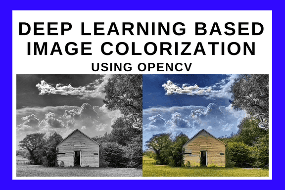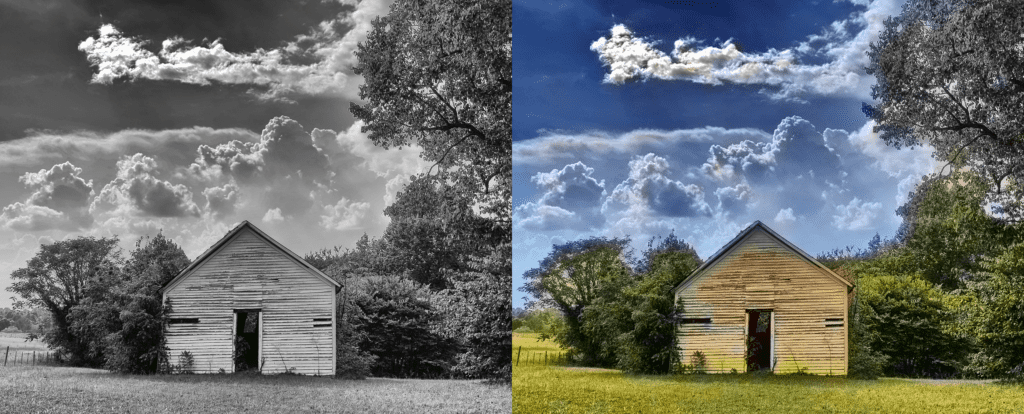
Sometimes technology enhances art. Sometimes it vandalizes it.
Colorizing black and white films is an ancient idea dating back to 1902. For decades many movie creators opposed the idea of colorizing their black-and-white movies and considered it vandalism of their art. Today it is accepted as an enhancement to the art form.
The technology itself has moved from painstaking hand colorization to today’s largely automated techniques. Legend Films used its automated technology to color old classics in the United States. In India, the movie Mughal-e-Azam, a blockbuster released in 1960, was remastered in color in 2004. People from multiple generations crowded the theatres to see it in color, and the movie was a huge hit for the second time!
Many colorization papers have been published using traditional computer vision methods. One of my favorites is a paper titled Colorization using Optimization by Anat Levin, Dani Lischinski, and Yair Weiss. It used a few colored scribbles to guide an optimization problem for solving colorization.
Wouldn’t it be cool if an algorithm did not use user input?
In the last few years, with the Deep Learning revolution, automation in colorization has taken a huge leap forward. In this post, we will learn about one such Deep Learning model. We also share OpenCV code to use the trained model in a Python or C++ application.
Colorful Image Colorization
In ECCV 2016, Richard Zhang, Phillip Isola, and Alexei A. Efros published a paper titled Colorful Image Colorization in which they presented a Convolutional Neural Network for colorizing gray images. They trained the network with 1.3M images from ImageNet training set. The authors have also made a trained Caffe-based model publicly available. In this post, we will first define the colorization problem, explain the paper’s architectural details, and share the code and some fascinating results.
If you are new to Deep Learning, we encourage you to review our introductory posts on Deep Learning first.
Defining the Colorization Problem
Let’s first define the colorization problem in terms of the CIE Lab color space. Like the RGB color space, it is a 3-channel color space, but unlike the RGB color space, color information is encoded only in the a (green-red component) and b (blue-yellow component) channels. The L (lightness) channel encodes intensity information only.
The grayscale image we want to color can be thought of as the L-channel of the image in the Lab color space, and our objective to find the a and b components. The Lab image so obtained can be transformed to the RGB color space using standard color space transforms. For example, in OpenCV, this can be achieved using cvtColor with COLOR_BGR2Lab option.
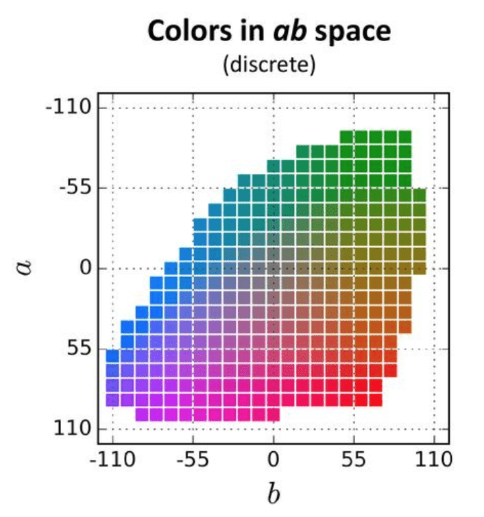
To simplify calculations, the ab space of the Lab color space is quantized into 313 bins as shown in Figure 2. Instead of finding the a and b values for every pixel, because of this quantization, we simply need to find a bin number between 0 and 312. Yet another way of thinking about the problem is that we already have the L channel that takes values from 0 to 255, and we need to find the ab channel that takes values between 0 to 312. So the color prediction task is now turned into a multinomial classification problem where for every gray pixel there are 313 classes to choose from.
CNN Architecture for Colorization
The architecture proposed by Zhang et al is a VGG-style network with multiple convolutional blocks. Each block has two or three convolutional layers followed by a Rectified Linear Unit (ReLU) and terminating in a Batch Normalization layer. Unlike the VGG net, there are no pooling or fully connected layers.
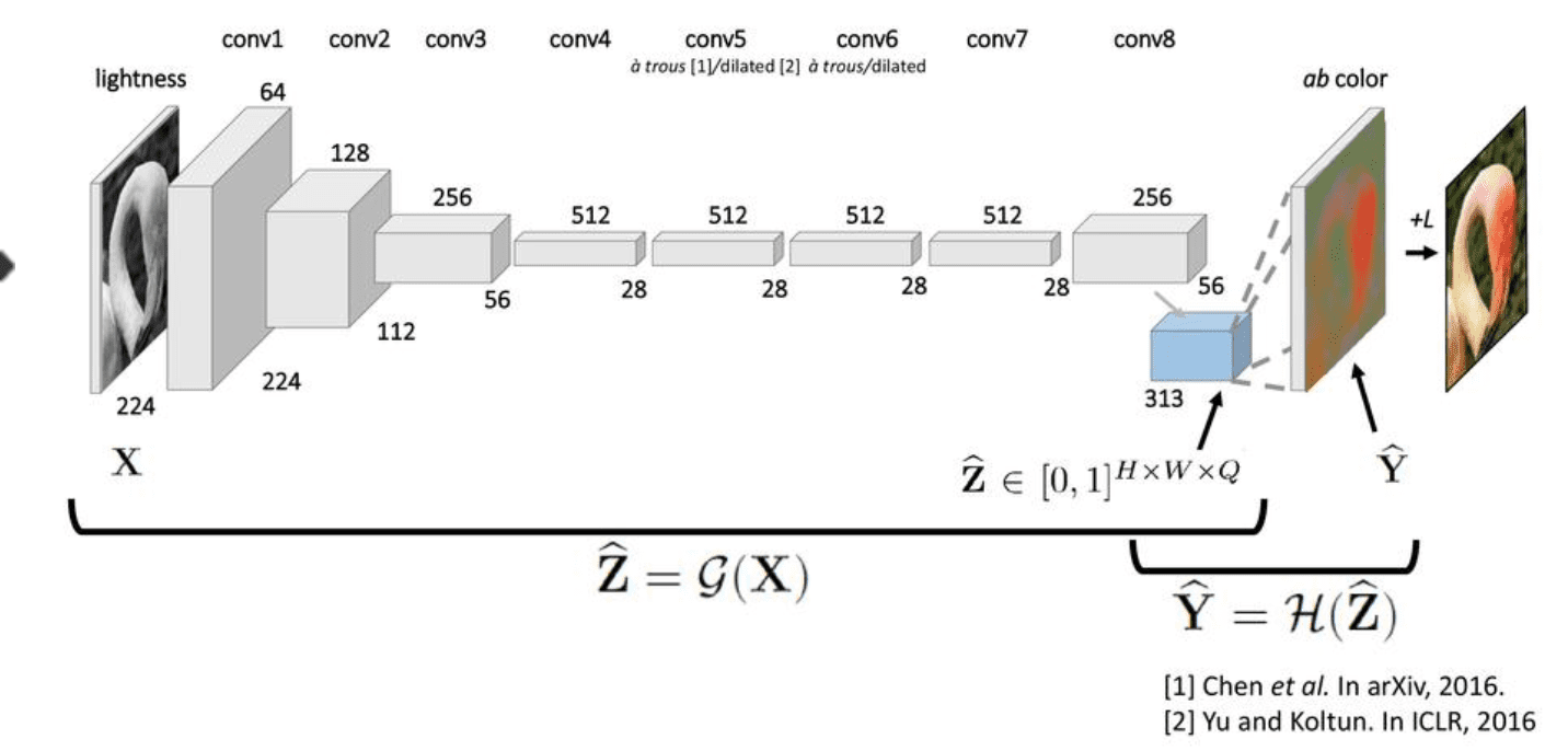
The input image is rescaled to 224×224. Let us represent this rescaled grayscale input image by ![]() .
.
When it passes through the neural network shown above, it gets transformed to ![]() by the neural network. Mathematically, this transformation
by the neural network. Mathematically, this transformation ![]() by the network can be written as
by the network can be written as
![]()
The dimensions of ![]() is
is ![]() x
x![]() x
x![]() , where
, where ![]() and
and ![]() are the height and width of the output of the last convolution layer. For each of the
are the height and width of the output of the last convolution layer. For each of the ![]() x
x![]() pixels,
pixels, ![]() contains a vector of
contains a vector of ![]() values where each value represents the probability of the pixel belonging to that class. We aim to find a single pair of ab channel values for each probability distribution
values where each value represents the probability of the pixel belonging to that class. We aim to find a single pair of ab channel values for each probability distribution ![]() .
.
Recovering color image from 
The CNN shown in Figure 3 gives us a collection of distributions in ![]() from the resized input image
from the resized input image ![]() . Let’s see how to recover a single ab value pair from each distribution in
. Let’s see how to recover a single ab value pair from each distribution in ![]() .
.
You may be tempted to think that we can take the mean of the distribution and choose the ab pair corresponding to the nearest quantized bin center. Unfortunately, this distribution is not Gaussian, and the mean of the distribution corresponds to an unnatural desaturated color. To understand this, think of the color of the sky — it is sometimes blue and sometimes orange-yellow. The distribution of colors of the sky is bi-modal. While coloring the sky, either blue or yellow will result in a plausible coloring. But the average of blue and yellow is an uninteresting gray.
So why not use the mode of the distribution so you get either blue or yellow sky? Sure, the authors tried that and while it gave vibrant colors, it sometimes broke spatial consistency. Their solution was to interpolate between the mean and mode estimates to obtain a quantity called the annealed-mean. A parameter called temperature (T) was used to control the degree of interpolation. A final value of T=0.38 is used as a trade-off between the two extremes.
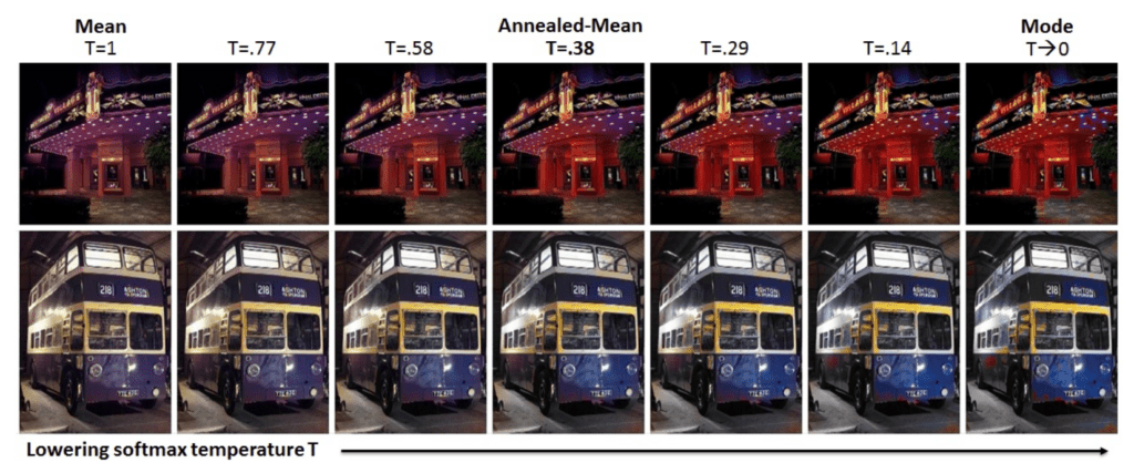
Figure 4: Annealed-mean using a temperature(T) is used to interpolate between the mean and mode of the distribution.
The ab pair corresponding to the annealed-mean of the distribution ![]() is represented in
is represented in ![]() , which can be written as a transformation of the original distribution
, which can be written as a transformation of the original distribution ![]()
![]()
Notice that when the image passes through the CNN, its size decreases to 56×56. Therefore the predicted ab image,
Multinomial Loss Function with Color Rebalancing
All Neural Networks are trained by defining a loss function. The goal of the training process is to minimize the loss over the training set. In the colorization problem, the training data consists of thousands of color images and their grayscale versions.
The output of the CNN is ![]() given an input image
given an input image ![]() . We need to transform all color images in the training set to their corresponding
. We need to transform all color images in the training set to their corresponding ![]() values. Mathematically, we simply want to invert the mapping
values. Mathematically, we simply want to invert the mapping ![]()
![]()
For every pixel, ![]() , of an output image
, of an output image ![]() we can simply find the nearest ab bin and represent
we can simply find the nearest ab bin and represent ![]() as a one-hot vector, in which we assign 1 to the nearest ab bin and 0 to all the other 312 bins. But for a better result, the 5-nearest neighbors are considered and a Gaussian distribution is used to compute the distribution
as a one-hot vector, in which we assign 1 to the nearest ab bin and 0 to all the other 312 bins. But for a better result, the 5-nearest neighbors are considered and a Gaussian distribution is used to compute the distribution ![]() depending on the distance from the ground truth.
depending on the distance from the ground truth.
If you have worked with CNNs before, you may be tempted to use the standard cross-entropy loss to compare the ground truth ![]() and the estimate
and the estimate ![]() using
using
![\[L(\hat{Z}, Z) = - \frac{1}{HW} \sum \limits_{h, w} \sum \limits_{q} Z_{h,w,q} \log (\hat{Z}_{h,w,q})\]](https://learnopencv.com/wp-content/ql-cache/quicklatex.com-35ea818bdbe39c41cd94b0e6a45e2803_l3.png)
The above loss function, unfortunately, produces very dull colors. This is because the distribution of colors in ImageNet is heavy around the gray line.
Color Rebalancing
To nudge the algorithm to produce vibrant colors, the authors changed the loss function to
![\[L(\hat{Z}, Z) = - \frac{1}{HW} \sum\limits_{h,w} v(Z_{h,w}) \sum\limits_{q}Z_{h,w,q} \log (\hat{Z}_{h,w,q})\]](https://learnopencv.com/wp-content/ql-cache/quicklatex.com-833917b4b78db6b1f9d0e164b3a6ce96_l3.png)
The color rebalancing term, ![]() is used to rebalance the loss based on the rarity of the color class. This contributes towards getting more vibrant and saturated colors in the output.
is used to rebalance the loss based on the rarity of the color class. This contributes towards getting more vibrant and saturated colors in the output.
Results of Colorization
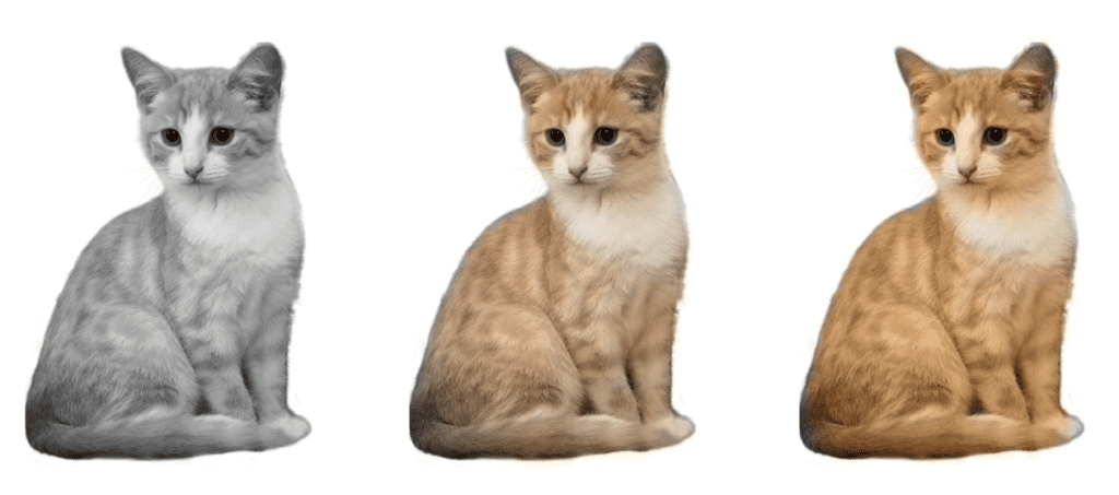
The authors have shared the trained Caffe models for both versions – with and without color rebalancing. We tried both version and have shared the results in the Figure below. The middle column shows the version without color rebalancing and the last column shows the version with rebalancing.
As we can see, color rebalancing makes many images very lively and vibrant. Most of them are plausible colors. On the other hand, sometimes it could also add some unwanted saturated color patches to some images.
Keep in mind that when we try to convert a grayscale image into a color image, there could be multiple plausible solutions. So the way to evaluate good colorization is not how well it matches the ground truth, but how plausible and pleasant it looks to the human eyes.
Animals
The model does very well on images of animals — especially cats and dogs. This is because ImageNet contains a very large collection of these animals.

Outdoor Scenes
The model also does a very good job of outdoor scenes showing blue sky and green vegetation. Also notice, given a silhouette of a tree, the model predicts an orange sky indicating the fact that it has captured the notion of sunset.


Sketches
Finally, even with sketches, the model produces plausible colorization.


Colorizing a Video
We also applied the colorization to a video and here is the result. We are also sharing the code for video colorization.
Implementing Image Colorization Using CNN With OpenCV
The authors have provided the pre-trained model and the network details in GitHub at this location. Below, we go over the Python and C++ code to colorize a given gray scale image using these pre-trained models. Our code is based on the OpenCV sample code. We used OpenCV version 3.4.1. We also provide code to colorize a given grayscale video.
Download model
Let’s start by downloading the models using the script file getModels.sh from command line.
sudo chmod a+x getModels.sh
./getModels.sh
This will download the .prototxt file (containing the network’s architecture), the trained caffe models for both with and without color rebalancing and the pts_in_hull.py file which has the center of the bins in the quantized ab space. In the C++ version, the center of the bins are copied from pts_in_hull.py.
Read model
Next, we provide the paths to the protoFile and the weightsFile in the code. Select the appropriate model, depending on whether you want to use color rebalancing or not. We have defaulted it to using the color rebalancing model. Read the input image and define the network’s input size to be 224×224. Read the network into memory.
Python
# Specify the paths for the model files
protoFile = "./models/colorization_deploy_v2.prototxt"
weightsFile = "./models/colorization_release_v2.caffemodel"
#weightsFile = "./models/colorization_release_v2_norebal.caffemodel";

# Read the input image
frame = cv.imread("./dog-greyscale.png")

W_in = 224
H_in = 224

# Read the network into Memory
net = cv.dnn.readNetFromCaffe(protoFile, weightsFile)
C++
// Specify the paths for the 2 files
string protoFile = "./models/colorization_deploy_v2.prototxt";
string weightsFile = "./models/colorization_release_v2.caffemodel";
//string weightsFile = "./models/colorization_release_v2_norebal.caffemodel";

Mat img = imread(imageFile);
const int W_in = 224;
const int H_in = 224;

// Read the network into Memory
Net net = readNetFromCaffe(protoFile, weightsFile);
Load quantized bin centers
Next, we load quantized bin centers. We then assign 1×1 kernels corresponding to each of the 313 bin centers and assign them to the corresponding layer in the network. Finally, we add a scaling layer with a non-zero value.
Python
# Load the bin centers
pts_in_hull = np.load('./pts_in_hull.npy')

# populate cluster centers as 1x1 convolution kernel
pts_in_hull = pts_in_hull.transpose().reshape(2, 313, 1, 1)
net.getLayer(net.getLayerId('class8_ab')).blobs = [pts_in_hull.astype(np.float32)]
net.getLayer(net.getLayerId('conv8_313_rh')).blobs = [np.full([1, 313], 2.606, np.float32)]
C++
// populate cluster centers as 1x1 convolution kernel
int sz[] = {2, 313, 1, 1};
const Mat pts_in_hull(4, sz, CV_32F, hull_pts);
Ptr<dnn::Layer> class8_ab = net.getLayer("class8_ab");
class8_ab->blobs.push_back(pts_in_hull);
Ptr<dnn::Layer> conv8_313_rh = net.getLayer("conv8_313_rh");
conv8_313_rh->blobs.push_back(Mat(1, 313, CV_32F, Scalar(2.606)));
Convert image to CIE Lab Color Space
The input RGB image is scaled so that the values are in the range 0-1, and then it is converted to Lab color space and the lightness channel is extracted out.
Python
#Convert the rgb values of the input image to the range of 0 to 1
img_rgb = (frame[:,:,[2, 1, 0]] * 1.0 / 255).astype(np.float32)
img_lab = cv.cvtColor(img_rgb, cv.COLOR_RGB2Lab)
img_l = img_lab[:,:,0] # pull out L channel
C++
Mat lab, L, input;
img.convertTo(img, CV_32F, 1.0/255);
cvtColor(img, lab, COLOR_BGR2Lab);
extractChannel(lab, L, 0);
The lightness channel in the original image is resized to the network input size which is (224,224) in this case. Usually, the lightness channel ranges from 0 to 100. So we subtract 50 to center it at 0.
Python
# resize the lightness channel to network input size
img_l_rs = cv.resize(img_l, (W_in, H_in)) # resize image to network input size
img_l_rs -= 50 # subtract 50 for mean-centering
C++
resize(L, input, Size(W_in, H_in));
input -= 50;
Then we feed the scaled and mean-centered lightness channel to the network as its input for the forward pass. The output of the forward pass is the predicted ab channel for the image. It is scaled back to the original image size and then merged with the original-sized lightness image(extracted earlier in original resolution) to get the output Lab image. It is then converted to RGB color space to get the final color image. We can then save the output image.
Python
net.setInput(cv.dnn.blobFromImage(img_l_rs))
ab_dec = net.forward()[0,:,:,:].transpose((1,2,0)) # this is our result

(H_orig,W_orig) = img_rgb.shape[:2] # original image size
ab_dec_us = cv.resize(ab_dec, (W_orig, H_orig))
img_lab_out = np.concatenate((img_l[:,:,np.newaxis],ab_dec_us),axis=2) # concatenate with original image L
img_bgr_out = np.clip(cv.cvtColor(img_lab_out, cv.COLOR_Lab2BGR), 0, 1)

cv.imwrite('dog_colorized.png', cv.resize(img_bgr_out*255, imshowSize))
C++
// run the L channel through the network
Mat inputBlob = blobFromImage(input);
net.setInput(inputBlob);
Mat result = net.forward();

// retrieve the calculated a,b channels from the network output and resize them to the original image size
Size siz(result.size[2], result.size[3]);
Mat a = Mat(siz, CV_32F, result.ptr(0,0));
Mat b = Mat(siz, CV_32F, result.ptr(0,1));
resize(a, a, img.size());
resize(b, b, img.size());

// merge and convert back to BGR
Mat color, chn[] = {L, a, b};
merge(chn, 3, lab);
cvtColor(lab, color, COLOR_Lab2BGR);
We encourage the reader to try out the video version of the code too.
References:
- Colorful Image Colorization, Richard Zhang, Phillip Isola, Alexei A. Efros, ECCV 2016
- OpenCV Samples on Colorization
- Images and videos used in this post are in the public domain and were obtained from the following sources: Wikimedia Commons, Maxpixel, pxhere, Pixabay [1], [2], [3], [4], [5] and Pexels


