In this post, we will learn what Batch Normalization is, why it is needed, how it works, and how to implement it using Keras.

Batch Normalization was first introduced by two researchers at Google, Sergey Ioffe and Christian Szegedy in their paper ‘Batch Normalization: Accelerating Deep Network Training by Reducing Internal Covariate Shift‘ in 2015. The authors showed that batch normalization improved the top result of ImageNet (2014) by a significant margin using only 7% of the training steps. Today, Batch Normalization is used in almost all CNN architectures.

In this post, we will first train a standard architecture shared in the Keras library example on the CIFAR10 dataset. We will then add batch normalization to the architecture and show that the accuracy increases significantly (by 10%) in fewer epochs.

Internal Covariate Shift

Before we jump into the nitty-gritty of batch normalization, let us first understand a basic principle in machine learning.

Let’s say we have a flower dataset and want to build a binary classifier for roses. The output is 1 if the image is that of a rose, and the output is 0 otherwise.

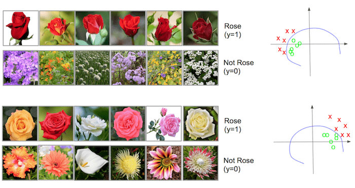
Consider a subset of the training data that primarily has red rose buds as rose and wildflowers as non-rose examples. These are shown in Figure 1.

Consider another subset, shown in Figure 2, that has fully blown roses of different colors as rose examples and other non-rose flowers in the picture as non-rose examples.

Intuitively, it makes sense that every mini-batch used in the training process should have the same distribution. In other words, a mini-batch should not have only images from one of the two subsets above. It should have images randomly selected from both subsets in each mini-batch.

The same intuition is graphically depicted in Figure 3. The last column of Figure 3 shows the two classes (roses and non-roses) in the feature space (shown in two dimensions for ease of visualization). The blue curve shows the decision boundary. We can see the two subsets lie in different regions of the feature space. This difference in distribution is called the covariate shift. When the mini-batches have images uniformly sampled from the entire distribution, there is negligible covariate shift. However, when the mini-batches are sampled from only one of the two subsets shown in Figure 1 and Figure 2, there is a significant covariate shift. This makes the training of the rose vs non-rose classifier very slow.

An easy way to solve this problem for the input layer is to randomize the data before creating mini-batches.

But how do we solve this for the hidden layers? Just as it made intuitive sense to have a uniform distribution for the input layer, it is advantageous to have the same input distribution for each hidden unit over time while training. But in a neural network, each hidden unit’s input distribution changes every time there is a parameter update in the previous layer. This is called internal covariate shift. This makes training slow and requires a minimal learning rate and a good parameter initialization. This problem is solved by normalizing the layer’s inputs over a mini-batch, which is called Batch Normalization.

By now, we have an intuitive sense of why Batch Normalization is a good idea. Now, let’s figure out how to do this normalization.

Batch Normalization in a Neural network

Batch normalization is done individually at each unit. Figure 4 shows how it works on a simple network with input features and . Don’t be overwhelmed by the notation! Let’s go over the equations.

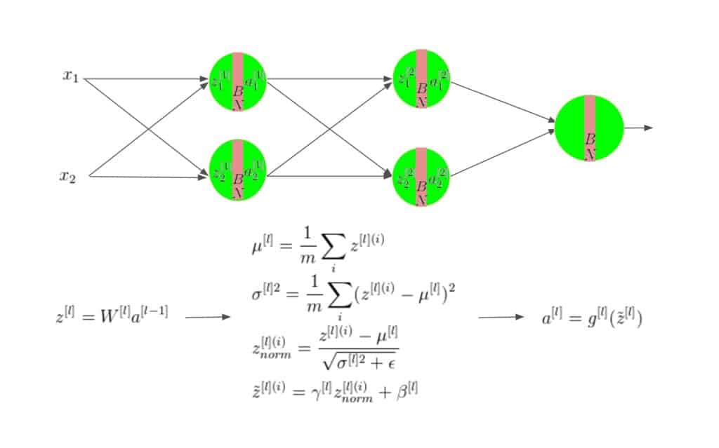
In Figure 4, the superscript corresponds to the data in the mini-batch, the superscript indicates the layer in the network, and the subscript indicates the dimension in a given layer in the network. In some places, either the superscripts or the subscript has been dropped to keep the notations simple.

Batch Normalization is done individually at every hidden unit. Traditionally, the input to a layer goes through an affine transform which is then passed through a non-linearity such as ReLU or sigmoid to get the final activation from the unit. So,

.

But when Batch Normalization is used with a transform , it becomes

The bias could now be ignored because its effect is subsumed with the shift parameter .

The four equations shown in Figure 4 do the following.

1. Calculate the mean () of the minibatch.
2. Calculate the variance () of the minibatch.
3. Calculate by subtracting mean from and subsequently dividing by standard deviation (). A small number, epsilon (), is added to the denominator to prevent dividing by zero.
4. Calculate by multiplying with a scale () and adding a shift () and use in place of as the non-linearity’s (e.g. ReLU’s) input. The two parameters and are learned during the training process with the weight parameters .

Note: Batch normalization adds only two extra parameters for each unit. So the representation power of the network is still preserved. If is set to and to , then equals , thus working as an identity function. Thus introducing batch normalization alone would not reduce the accuracy because the optimizer still has the option to select no normalization effect using the identity function, and it would be used by the optimizer only to improve the results.

Other benefits of Batch Normalization

Higher learning rate

If we use a high learning rate in a traditional neural network, the gradients could explode or vanish. Large learning rates can scale the parameters, which could amplify the gradients, thus leading to an explosion. But if we do batch normalization, small changes in parameters to one layer do not get propagated to other layers. This makes it possible to use higher learning rates for the optimizers, which otherwise would not have been possible. It also makes gradient propagation in the network more stable.

Adds Regularization

Since the normalization step sees all the training examples in the mini-batch together, it brings in a regularization effect with it. If batch normalization is performed through the network, then the dropout regularization could be dropped or reduced in strength.

Makes it possible to use saturating non-linearities

In traditional deep neural networks, it is very hard to use saturating activation functions like the sigmoid, where the gradient is close to zero for inputs outside the range (-1,1). The change in parameters in the previous layers can easily throw the activation function’s inputs close to these saturating regions, and the gradients could vanish. This problem is worse in deeper networks. On the other hand, if the distribution of the inputs to these nonlinearities remains stable, then it would save the optimizer from getting stuck in the saturated regions, and thus training would be faster.

Batch Normalization in Keras

We use the Keras code provided here as a baseline for showing how batch normalizations can improve accuracy by a large margin. The baseline code does not use batch normalization, and the following changes were made to it to add on batch normalization.

Click here to download the source code to this post

Import the BatchNormalization modules from Keras layers

from keras.layers import BatchNormalization

Batch Normalization calls were added in Keras after the Conv2D or Dense function calls but before the following Activation function calls. Here are some examples.

model.add(Conv2D(32, (3, 3)))
model.add(BatchNormalization())
model.add(Activation('relu'))

model.add(Dense(32, (3, 3)))
model.add(BatchNormalization())
model.add(Activation('relu'))

Dropout calls were removed. Batch Normalization itself has some regularization effect. So usually, dropouts can be reduced. In our case, removing it altogether also did not reduce accuracy. The learning rate of the optimizer was increased 10 times from 0.0001 to 0.001. Rmsprop optimizer was used as in the baseline code, but this would be true for other optimizers. We used the same numpy seed for both the baseline and batch normalization versions to make a fair comparison between the two output versions. Since most of the deep learning algorithms are stochastic, their outputs are not exactly the same in different runs, but the batch normalization version outperformed the baseline version by large margins in all the runs, with the same numpy seed as well as without giving the same numpy seed.

from numpy.random import seed
seed(7)

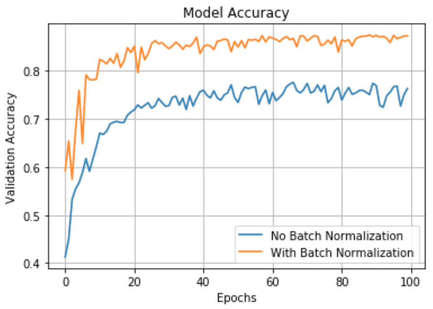
Both versions have roughly the same run time needed for each epoch (24-25 s), but as we see in the above plot, the accuracy attains a much higher value much faster if we use batch normalization. The Keras team reports an accuracy of  79% after 50 epochs, as seen in their Github code. Our run of the same code gave a maximum accuracy of 77%, which seems fair, given it is in the same range as theirs and the stochastic nature of the Keras runs. But with batch normalization, it increases to 87%. All these runs were done on a GeForce GTX 1080.

Above is the plot of the validation vs training losses for both versions. As we can see, the validation loss reduces substantially with batch normalization.

References

1. Paper : Batch Normalization: Accelerating Deep Network Training by Reducing Internal Covariate Shift by Sergecody Ioffe and Christian Szegedy, 2015
2. Inspiration : Coursera course on “Improving Deep Neural Networks: Hyperparameter tuning, Regularization and Optimization“, Week 3. Deep Learning Specialization by Andrew Ng, deeplearning.ai
3. Image Credits : Some of the flower images used in this post were originally provided by Amanda, Jonathan & Hannes Grobe under the CC BY-SA 2.5 license, from Wikimedia Commons.