Activation Functions in Deep Learning

This post is part of the series on Deep Learning for Beginners, which consists of the following tutorials :

In this post, we will learn about different activation functions in Deep learning and see which activation function is better than the other. This post assumes that you have a basic idea of Artificial Neural Networks (ANN), but in case you don’t, I recommend you first read the post on understanding feedforward neural networks.

1. What is an Activation Function?

Biological neural networks inspired the development of artificial neural networks. However, ANNs are not even an approximate representation of how the brain works. It is still useful to understand the relevance of an activation function in a biological neural network before we know why we use it in an artificial neural network.

A typical neuron has a physical structure that consists of a cell body, an axon that sends messages to other neurons, and dendrites that receives signals or information from other neurons.

In the above picture, the red circle indicates the region where the two neurons communicate. The neuron receives signals from other neurons through the dendrites. The weight (strength) associated with a dendrite, called synaptic weights, gets multiplied by the incoming signal. The signals from the dendrites are accumulated in the cell body, and if the strength of the resulting signal is above a certain threshold, the neuron passes the message to the axon. Otherwise, the neuron kills the signal and is not propagated further.

The activation function makes the decision of whether or not to pass the signal. In this case, it is a simple step function with a single parameter – the threshold. Now, when we learn something new ( or unlearn something ), the threshold and the synaptic weights of some neurons change. This creates new connections among neurons making the brain learn new things.

Let us understand the same concept again but this time using an artificial neuron.

In the above figure, $(x_1, \cdots , x_n)$ is the signal vector that gets multiplied with the weights $\left( w_1, w_2, \cdots, w_n \right)$ . This is followed by accumulation ( i.e., summation + addition of bias $b$ ). Finally, an activation function $f$ is applied to this sum.

Note that the weights $\left( w_1, w_2, \cdots, w_n \right)$ and the bias $b$ transform the input signal linearly. The activation, on the other hand, transforms the signal non-linearly. This non-linearity allows us to learn arbitrarily complex transformations between the input and the output.

Over the years, various functions have been used, and it is still an active area of research to find a proper activation function that makes the neural network learn better and faster.

2. How Does the Network Learn? – Activation Functions in Deep Learning

Getting a basic idea of how the neural network learns is essential. Let’s say that the desired output of the network is $y$ . The network produces an output $y'$ . The difference between the predicted and desired output $(y - y)$ is converted to a metric known as the loss function ( $J$ ). The loss is high when the neural network makes a lot of mistakes, and it is low when it makes fewer mistakes. The training process aims to find the weights and biases that minimize the loss function over the training set.

In the figure below, the loss function is shaped like a bowl. At any point in the training process, the partial derivatives of the loss function w.r.t to the weights is nothing but the slope of the bowl at that location. One can see that by moving in the direction predicted by the partial derivatives, we can reach the bottom of the bowl and therefore minimize the loss function. This idea of using the partial derivatives of a function to iteratively find its local minimum is called gradient descent.

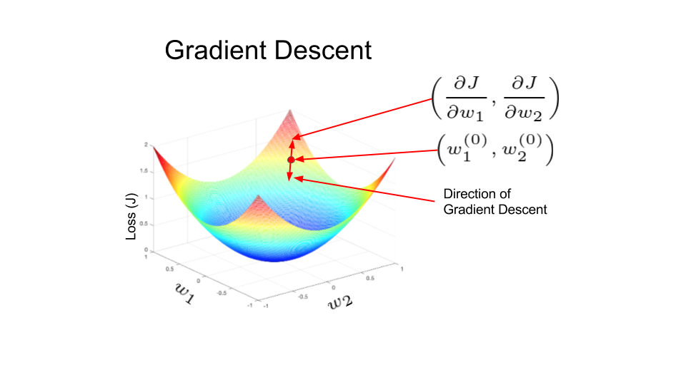
In Artificial neural networks, the weights are updated using a method called Backpropagation. The partial derivatives of the loss function w.r.t the weights are used to update the weights. In a sense, the error is backpropagated in the network using derivatives. This is done iteratively and after many iterations, the loss reaches a minimum value, and the derivative of the loss becomes zero.

We plan to cover backpropagation in a separate post. The main thing to note here is the presence of derivatives in the training process.

3. Types of Activation Functions

Linear Activation Function: It is a simple linear function of the form $f(x) = x$ Basically, the input passes to the output without any modification.

linear activation functions — Figure Linear Activation Function

Non-Linear Activation Functions: These functions are used to separate the data that is not linearly separable and are the most used activation functions. A non-linear equation governs the mapping from inputs to outputs. A few examples of different types of non-linear activation functions are sigmoid, tanh, relu, lrelu, prelu, swish, etc. We will be discussing all these activation functions in detail.

4. Why do we Need a Non-Linear Activation Function in an Artificial Neural Network?

Neural networks are used to implement complex functions, and non-linear activation functions enable them to approximate arbitrarily complex functions. Without the non-linearity introduced by the activation function, multiple layers of a neural network are equivalent to a single-layer neural network.

Let’s see a simple example to understand why without non-linearity, it is impossible to approximate even simple functions like XOR and XNOR gate. In the figure below, we graphically show an XOR gate. There are two classes in our dataset represented by a cross and a circle. When the two features, $X1$ and $X2$ are the same, the class label is a red cross; otherwise, it is a blue circle. The two red crosses have an output of 0 for input values (0,0) and (1,1), and the two blue rings have an output of 1 for input values (0,1) and (1,0).

xor – LearnOpenCV — Figure Graphical Representation of XOR gate

From the above picture, we can see that the data points are not linearly separable. In other words, we can not draw a straight line to separate the blue circles and the red crosses from each other. Hence, we will need a non-linear decision boundary to separate them.

The activation function is also crucial for squashing the output of the neural network to be within certain bounds. The output of a neuron $\sum^n_i w_i x_i + b$ can take on very large values. This output, when fed to the next layer neuron without modification, can be transformed to even larger numbers thus making the process computationally intractable. One of the tasks of the activation function is to map the output of a neuron to something that is bounded ( e.g., between 0 and 1).

With this background, we are ready to understand different types of activation functions.

5. Types of Non-Linear Activation Functions

5.1. Sigmoid

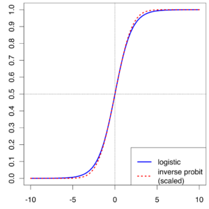
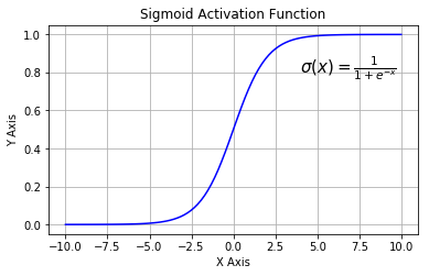
It is also known as Logistic Activation Function. It takes a real-valued number and squashes it into a range between 0 and 1. It is also used in the output layer, where our end goal is to predict probability. It converts large negative numbers to 0 and large positive numbers to 1. Mathematically it is represented as

$\sigma(x) = \frac{1}{1 + e^{-x}}$

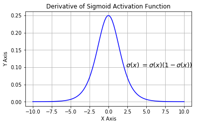
The figure below shows the sigmoid function and its derivative graphically

sigmoid activation funstions — Figure Sigmoid Activation Function

sigmond derivative — Figure Sigmoid Derivative

The three major drawbacks of sigmoid are:

Vanishing gradients: Notice the sigmoid function is flat near 0 and 1. In other words, the gradient of the sigmoid is 0 near 0 and 1. During backpropagation through the network with sigmoid activation, the gradients in neurons whose output is near 0 or 1 are nearly 0. These neurons are called saturated neurons. Thus, the weights in these neurons do not update. Not only that, the weights of neurons connected to such neurons are also slowly updated. This problem is also known as a vanishing gradient. So, imagine if there was a large network comprising of sigmoid neurons in which many of them are in a saturated regime; then the network will not be able to backpropagate.
Not zero-centered: Sigmoid outputs are not zero-centered.
Computationally expensive: The exp() function is computationally expensive compared with the other non-linear activation functions.

The next non-linear activation function that I will discuss addresses the zero-centered problem in sigmoid.

5.2. Tanh

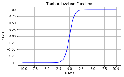
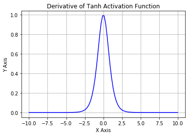
tanh – LearnOpenCV — Figure Tanh Activation Function

It is also known as the hyperbolic tangent activation function. Like sigmoid, tanh also takes a real-valued number but squashes it into a range between -1 and 1. Unlike sigmoid, tanh outputs are zero-centered since the scope is between -1 and 1. You can think of a tanh function as two sigmoids put together. In practice, tanh is preferable over sigmoid. The negative inputs are considered as strongly negative, zero input values mapped near zero, and the positive inputs are regarded as positive. The only drawback of tanh is:

The tanh function also suffers from the vanishing gradient problem and therefore kills gradients when saturated.

To address the vanishing gradient problem, let us discuss another non-linear activation function known as the rectified linear unit (ReLU), which is much better than the previous two activation functions and is most widely used.

5.3. Rectified Linear Unit (ReLU)

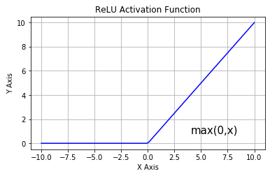
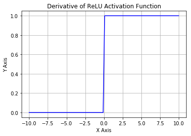
Relu Derivative — Figure ReLU Derivative

ReLU is half-rectified from the bottom, as shown in the figure above. Mathematically, it is given by this simple expression.

$f(x) = \max(0,x)$

This means that when the input x < 0 the output is 0; if x > 0 the output is x. This activation makes the network converge much faster. It does not saturate, which means it is resistant to the vanishing gradient problem at least in the positive region ( when x > 0), so the neurons do not backpropagate all zeros at least in half of their regions. ReLU is computationally very efficient because it is implemented using simple thresholding. But there are few drawbacks of ReLU neuron :

Not zero-centered: The outputs are not zero centered similar to the sigmoid activation function.
The other issue with ReLU is that if x < 0 during the forward pass, the neuron remains inactive and it kills the gradient during the backward pass. Thus weights do not get updated, and the network does not learn. When x = 0 the slope is undefined at that point, but this problem is taken care of during implementation by picking either the left or the right gradient.

To address the vanishing gradient issue in ReLU activation function when x < 0 we have something called Leaky ReLU which was an attempt to fix the dead ReLU problem. Let’s understand leaky ReLU in detail.

5.4. Leaky ReLU

leaky RELU activation fiunctions - Activation functions in deep learning — Figure Leaky ReLU activation function

This was an attempt to mitigate the dying ReLU problem. The function computes

$f(x) = max(0.1x, x)$

The concept of leaky ReLU is when x < 0, it will have a small positive slope of 0.1. This function somewhat eliminates the dying ReLU problem, but the results achieved with it are not consistent. Though it has all the characteristics of a ReLU activation function, i.e., computationally efficient, it converges much faster but does not saturate in the positive regions.

The idea of leaky ReLU can be extended even further. Instead of multiplying x with a constant term, we can multiply it with a hyperparameter which seems to work better with the leaky ReLU. This extension to leaky ReLU is known as Parametric ReLU.

5.5. Parametric ReLU

The PReLU function is given by

$f(x) = \max(\alpha x, x)$

Where $\alpha$ is a hyperparameter. The idea here was to introduce an arbitrary hyperparameter $\alpha$ , and this $\alpha$ can be learned since you can backpropagate into it. This gives the neurons the ability to choose what slope is best in the negative region, and with this ability, they can become a ReLU or a leaky ReLU.

In summary, it is better to use ReLU, but you can experiment with Leaky ReLU or Parametric ReLU to see if they give better results for your problem

5.6. SWISH

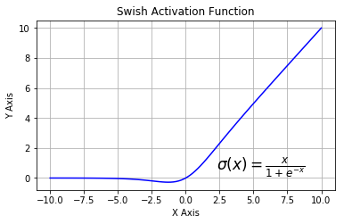
Activation functions in deep learning — Figure SWISH Activation Function

Also known as a self-gated activation function, has recently been released by researchers at Google. Mathematically it is represented as

$\sigma(x) = \frac{x}{1 + e^{-x}}$

According to the Self-Gated Activation Function paper, the SWISH activation function performs better than ReLU

From the above figure, we can observe that in the negative region of the x-axis the shape of the tail is different from the ReLU activation function, and because of this, the output from the Swish activation function may decrease even when the input value increases. Most activation functions are monotonic, i.e., their value never decreases as the input increases. Swish has one-sided boundedness property at zero; it is smooth and is non-monotonic. It will be interesting to see how well it performs by changing just one line of code.

Activation Functions in Deep Learning – A Complete Overview