Using Facial Landmarks for Overlaying Faces with Masks

Have you ever wondered how Instagram masks are fitting so perfectly on your face? Would you like to know how you can try to implement something similar by yourself? This post will help you with that! We will discuss using Facial Landmarks for Overlaying Faces with Masks.

To remind you how important it is to wear a medical mask in the current COVID-19 pandemic, we will write a demo script that overlays your face captured from a camera with a virtual medical mask using facial landmarks. You won’t only learn how this could be done with the help of computer vision, but also can try out different masks yourself. Oh, and don’t forget to wear a real mask to protect yourself once you are in public! Stay safe, and stay tuned.

Getting Started

To write a demo, we should discuss its pipeline and break our big task into smaller ones. Here’s what our algorithm will do step by step:

1. Find a face on the image.
2. Detect specific landmarks on a face.
3. Overlay the image with a mask.

Let’s discuss each of these steps in more detail.

Face Detection

First of all, to apply a facial mask, we should be aware of the face location on the image. How we can find a face? That’s easy, OpenCV will help us! We will use the DNN module of the OpenCV library, which we’ve already used in one of our earlier posts. OpenCV provides a simple API, to the underlying deep learning models. To use them we only need two files – one with the model architecture, the other one is with trained weights. We’ve got the ones from the OpenCV samples, you can find them in the detection folder with the rest of our code. Here’s the code to obtain face detections:

Click here to download the source code to this post

# defining prototxt and caffemodel paths
detector_model = args.detector_model
detector_weights = args.detector_weights

# load model
detector = cv2.dnn.readNetFromCaffe(detector_model, detector_weights)
capture = cv2.VideoCapture(0)

while True:
    # capture frame-by-frame
    success, frame = capture.read()

    #...

    # get frame's height and width
    height, width = frame.shape[:2]  # 640×480

    # resize and subtract BGR mean values, since Caffe uses BGR images for input
    blob = cv2.dnn.blobFromImage(
        frame, scalefactor=1.0, size=(300, 300), mean=(104.0, 177.0, 123.0),
    )
    # passing blob through the network to detect a face
    detector.setInput(blob)
    # detector output format:
    # [image_id, class, confidence, left, bottom, right, top]
    face_detections = detector.forward()

Finding Facial Landmarks

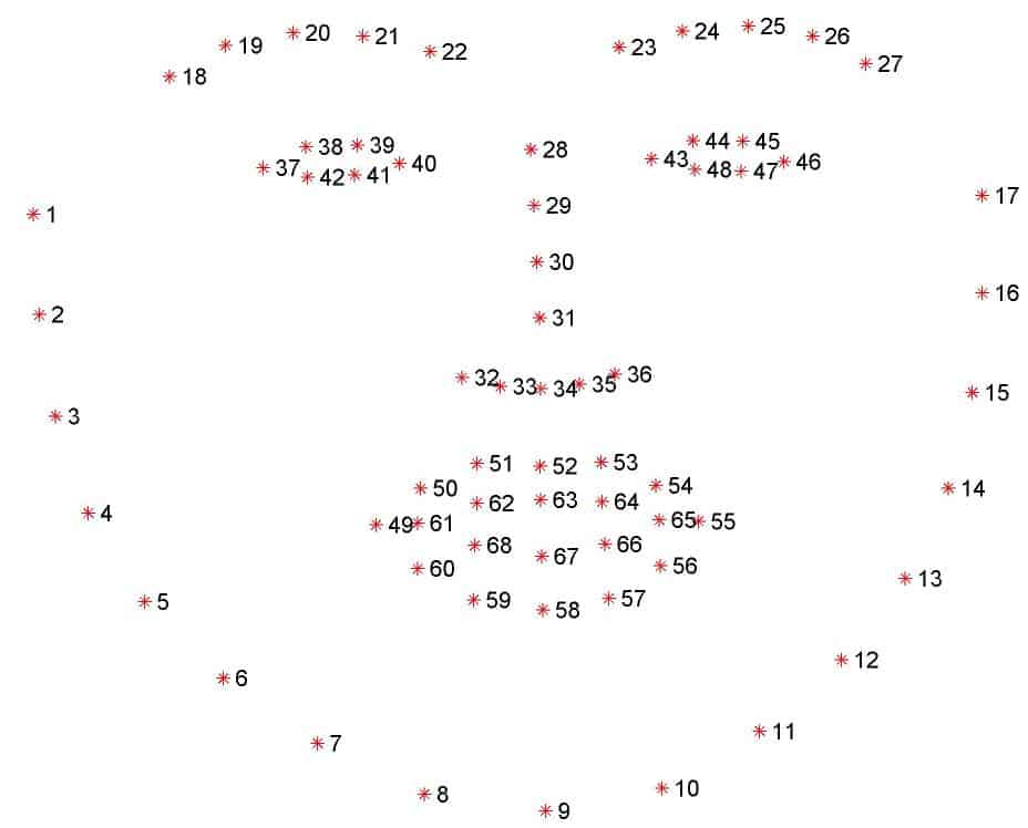
Now, when we got predicted bounding boxes with faces, we can use them as an input to the facial landmark detection network. The latter, in its turn, will output the key points that represent such face regions as eyes, eyebrows, nose, mouth, and jawline. Different approaches use a different amount of landmarks to describe face regions. We will be using 68 landmarks. You can find their visualization below:

If you’d like to know how to make it using classical computer vision algorithms, you can take a look at one of our posts, where we’ve done it. Here we will be using a deep-learning-based method, which is called
High-resolution networks (HRNet) for facial landmark detection.

We won’t dig deep into the details of this method. All we want from it is to input our detected face and get back 68 landmarks. If you’d like to find out more, please refer to the original paper, we provided the link above. Here’s the code below, how we should pre-process the output prediction from the detector to feed it to the HRNet:

# loop over the detections
for i in range(0, face_detections.shape[2]):
    # extract confidence
    confidence = face_detections[0, 0, i, 2]

    # filter detections by confidence greater than the minimum threshold
    if confidence > 0.5:
        # get coordinates of the bounding box from
        box = face_detections[0, 0, i, 3:7] * np.array([width, height, width, height])
        (x1, y1, x2, y2) = box.astype("int")

        # show original image
        cv2.imshow("original image", frame)

        # crop to detection and resize
        resized = crop(
            frame,
            torch.Tensor([x1 + (x2 - x1) / 2, y1 + (y2 - y1) / 2]),
            1.5,
            tuple(input_size),
        )

        # convert from BGR to RGB since HRNet expects RGB format
        resized = cv2.cvtColor(resized, cv2.COLOR_BGR2RGB)
        img = resized.astype(np.float32) / 255.0
        # normalize landmark net input
        normalized_img = (img - mean) / std

        # predict face landmarks
        model = model.eval()
        with torch.no_grad():
            input = torch.Tensor(normalized_img.transpose([2, 0, 1]))
            input = input.to(device)
            output = model(input.unsqueeze(0))
            score_map = output.data.cpu()
            preds = decode_preds(
                score_map,
                [torch.Tensor([x1 + (x2 - x1) / 2, y1 + (y2 - y1) / 2])],
                [1.5],
                score_map.shape[2:4],
            )

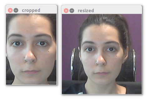
You should pay attention to how we resize the detected face. Since bounding boxes from the detector could sometimes be too tight, we do not crop the face from the original image precisely using the coordinates of the bounding box. Instead, we first scale the image, using scale factor 1.5, and then crop 256×256 sized image relatively to the center of the bounding box. That gives us a little richer face region:

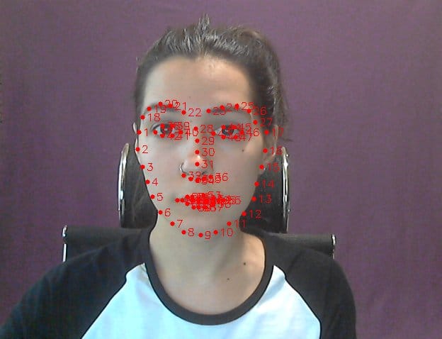
After pre-processing we use this image as the input to obtain the output score map with predicted landmarks. One more thing is that we can’t use these predictions as is, we need to decode them first with decode_preds function. What it does is to transform the landmark coordinates from the “score map coordinate system” to the original image, with respect to the same scaling we did to the input. The original image with the visualized landmarks will look like this:

Overlaying Image with a Mask

Now, when we have more representative information about the face and its parts, it will be quite easy to use it. Since a mask should cover the jawline at the bottom and nose at the top, we will be using landmarks from 2 to 16 and 30 from the nose. The next step is to apply a mask according to the landmarks.

Annotating Key Points on the Mask Image

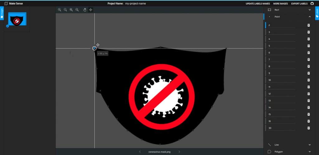
For better alignment, we need to annotate mask points that correspond to the chosen landmarks from the face. Different tools allow performing such annotation, we used an open-source online tool which is called makesense. It has an intuitive interface and makes it quite easy to work with. Here’s an
example of how the annotation for one of the masks looks like:

After you’ve done with the annotation, you need to save it to the .csv file:

All the mask images, that we use in our demo, are already annotated and have the corresponding file names with .csv extension as annotations.

Following the same steps, you can annotate your masks in .png and try them also!

Apply Mask using facial landmarks

The last and the final step is to apply the mask. Here’s the code that does it:

    # get chosen landmarks 2-16, 30 as destination points
    # note that landmarks numbering starts from 0
    dst_pts = np.array(
        [
            landmarks[1],
            landmarks[2],
            landmarks[3],
            landmarks[4],
            landmarks[5],
            landmarks[6],
            landmarks[7],
            landmarks[8],
            landmarks[9],
            landmarks[10],
            landmarks[11],
            landmarks[12],
            landmarks[13],
            landmarks[14],
            landmarks[15],
            landmarks[29],
        ],
        dtype="float32",
    )

    # load mask annotations from csv file to source points
    mask_annotation = os.path.splitext(os.path.basename(args.mask_image))[0]
    mask_annotation = os.path.join(
        os.path.dirname(args.mask_image), mask_annotation + ".csv",
    )

    with open(mask_annotation) as csv_file:
        csv_reader = csv.reader(csv_file, delimiter=",")
        src_pts = []
        for i, row in enumerate(csv_reader):
            # skip head or empty line if it's there
            try:
                src_pts.append(np.array([float(row[1]), float(row[2])]))
            except ValueError:
                continue
    src_pts = np.array(src_pts, dtype="float32")

    # overlay with a mask only if all landmarks have positive coordinates:
    if (landmarks > 0).all():
        # load mask image
        mask_img = cv2.imread(args.mask_image, cv2.IMREAD_UNCHANGED)
        mask_img = mask_img.astype(np.float32)
        mask_img = mask_img / 255.0

        # get the perspective transformation matrix
        M, _ = cv2.findHomography(src_pts, dst_pts)

        # transformed masked image
        transformed_mask = cv2.warpPerspective(
            mask_img,
            M,
            (result.shape[1], result.shape[0]),
            None,
            cv2.INTER_LINEAR,
            cv2.BORDER_CONSTANT,
        )

        # mask overlay
        alpha_mask = transformed_mask[:, :, 3]
        alpha_image = 1.0 - alpha_mask

        for c in range(0, 3):
            result[:, :, c] = (
                alpha_mask * transformed_mask[:, :, c]
                + alpha_image * result[:, :, c]
            )

# display the resulting frame
cv2.imshow("image with mask overlay", result)

We use findHomography function from the OpenCV library to find the transform between matched keypoints and then apply the found transformation matrix with prespectiveTransform function to map these points. If you’d like to find out more about what a homography is and where you can use it, take a look at our other posts here and here.

After applying the mentioned functions we have a new mask image the same size as the original one, with which we should overlay the original image. Since we’re using a mask image in .png format, it has a transparent alpha channel, which we use to merge both images into one.

Results

You can take a look at how our demo works with different masks:

Limitations of facial landmarks

Since we only have masks in frontal position and use wrap perspective function to match facial landmarks with the mask annotations, the algorithm doesn’t work correctly in cases of:

1. side view face
2. rotated in the 3D face, since we don’t use a 3D rotation matrix to perform points matching.