

In the previous post, we learned how to apply a fixed number of tags to images.
Let’s now switch to this broader task and see how we can tackle it.
In many real-life tasks, there is a set of possible classes (also called tags) for data, and you would like to find some subset of labels for each sample, not just a single label. This is often the case with text, image or video, where the task is to assign several most suitable labels to a particular text, image or video. We’re going to name this task multi-label classification throughout the post, but image (text, video) tagging is also a popular name for this task.
Multi-Label Classification
First, we need to formally define what multi-label classification means and how it is different from the usual multi-class classification. According to scikit-learn, multi-label classification assigns to each sample a set of target labels, whereas multi-class classification makes the assumption that each sample is assigned to one and only one label out of the set of target labels. Another way to look at it is that in multi-label classification, labels for each sample are just not mutually exclusive.
In the previous post, we also looked into the classification problem that handles multiple labels per sample. The key difference is that multi-output classification always predicts a fixed-length set of labels per sample and can be theoretically replaced with the corresponding number of separate classifiers while multi-label classification requires predicting non-fixed length subset of labels. Multi-output classification essentially answers several independent questions with one and only one possible answer for each.
To summarize differences between classification types let’s take a look at this photo. For each type of classification task, namely standard multi-class, multi-output and multi-label, there are different sets of possible labels and different predictions.


| Type | Predicted labels | Possible labels |
|---|---|---|
| Multi-class classification | smiling | [neutral, smiling, sad] |
| Multi-output classification | woman, smiling, brown hair | [man, woman, child] [neutral, smiling, sad] [brown hair, red hair, blond hair, black hair] |
| Multi-label classification | portrait, woman, smiling, brown hair, wavy hair | [portrait, nature, landscape, selfie, man, woman, child, neutral emotion, smiling, sad, brown hair, red hair, blond hair, black hair] |
As a real-life example, think about Instagram tags. People assign images with tags from some pool of tags (let’s pretend for the sake of example that this set is actually fixed). Tags are not mutually exclusive, they may represent what’s depicted on the image (e.g. “woman”, “wavy hair”, “smiling girl”, “cool shirt”) or some high-level concept (e.g. “portrait”, “happiness”, “fun”).
Let’s now try to tackle a similar problem by ourselves.
Data overview
We propose to use a part of the NUS-WIDE dataset as a toy problem in this post. It contains images annotated with a set of labels each.
Look at the example below:


You can download the dataset from the official site. NUS-WIDE contains images from Flickr (in fact, their URLs) with more than 1000 different labels. The set of labels was narrowed down by authors to 81 relevant ones.
Split data
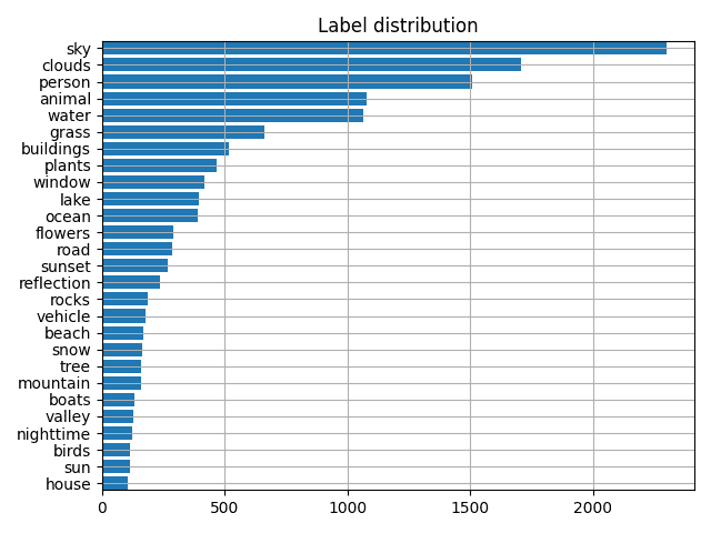
This dataset contains ~170k samples in total and is highly imbalanced. For some labels like “sky” and “clouds” there are ~61000 and ~45000 data samples, while for others like “map” or “earthquake” there are only 50.
Since the main purpose of this post is to demonstrate how to deal with multi-label classification, let’s try to make our life a bit easier and solve one task at a time. In order to do that, we decided to keep only the 27 most frequent labels so that each label has more than 100 corresponding samples. Also, for fast training, we took the first 6000 samples from the dataset. We split them to train and test subsets using a 5 to 1 ratio. The resulting size of the training set is 5000 images, and the test set – 1000 images.
Since NUS-WIDE is distributed as a list of URLs, it may be inconvenient to get the data as some links may be invalid. To save you this work, the author of this github repo shared already downloaded images. The whole dataset we’re using in this post can be downloaded here. You also can find the script to pre-process the annotation near the full code for this post (see below).
Dataset implementation and structure
The Pytorch’s Dataset implementation for the NUS-WIDE is standard and very similar to any Dataset implementation for a classification dataset. The input image size for the network will be 256×256. We also apply a more or less standard set of augmentations during training.
The entire annotation for 81 labels stored in nus_wide/train.json and nus_wide/test.json.
The subset annotation for 27 labels stored in nus_wide/small_train.json and nus_wide/small_test.json.
Each annotation file looks like:
[
    'samples':
        [
            {'image_name': '51353_2739084573_16e9be31f5_m.jpg' , 'image_labels': ['clouds', 'sky']}
            ...
        ]
    'labels' : ['house', 'birds', 'sun', 'valley', 'nighttime', 'boats', ...]
]
Model overview
As a backbone, we will use the standard ResNeXt50 architecture from torchvision. We’ll modify its output layer to apply it to our multi-label classification task.
Instead of 1000 classes (as in ImageNet), we will only have 27. We will also replace the softmax function with a sigmoid, let’s talk about why.

# Use the torchvision's implementation of ResNeXt, but add FC layer for a different number of classes (27) and a Sigmoid instead of a default Softmax.
class Resnext50(nn.Module):
    def __init__(self, n_classes):
        super().__init__()
        resnet = models.resnext50_32x4d(pretrained=True)
        resnet.fc = nn.Sequential(
            nn.Dropout(p=0.2),
            nn.Linear(in_features=resnet.fc.in_features, out_features=n_classes)
        )
        self.base_model = resnet
        self.sigm = nn.Sigmoid()

    def forward(self, x):
        return self.sigm(self.base_model(x))

# Initialize the model
model = Resnext50(len(train_dataset.classes))
# Switch model to the training mode
model.train()
Specific loss definition
We’ve chosen the dataset, the model architecture. The only thing left is the loss function, and since this is a classification problem, the choice may seem obvious – the CrossEntropy loss. Let’s see why we actually cannot use it for the multi-label classification problem.
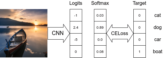
Here is how we calculate CrossEntropy loss in a simple multi-class classification case when the target labels are mutually exclusive. During the loss computation, we only care about the logit corresponding to the truth target label and how large it is compared to other labels.
In this example, the loss value will be -log(0.08) = 2.52.
Softmax makes all predicted probabilities sum to 1, so there couldn’t be several correct answers.
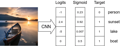
The obvious solution here is to treat each prediction independently. For example, using the Sigmoid function as a normalizer for each logit value separately.
Here we have several correct labels and predicted probability for each label. Now we can compare these probabilities with the probabilities of the correct labels (ones) using BinaryCrossEntropy loss.
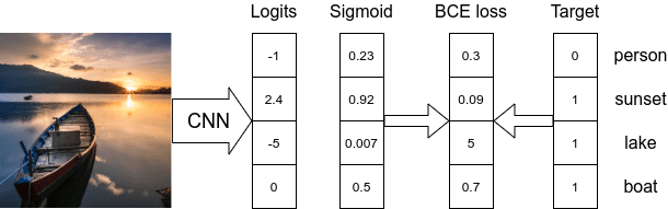
So the obvious solution is to use BinaryCrossEntropy loss. We define it in code simply as:
criterion = nn.BCELoss()
The only question left is what should we do with the predicted probabilities during the inference. The common thing to do is specifying a threshold value, so all labels with probabilities higher than it are considered predicted labels and others are skipped. We are using a threshold value of 0.5.
Metrics
We will use sklearn.metrics.precision_score (as well as recall_score and f1_score) with parameter average=’macro’, average=’micro’ or average=’samples’ to calculate metrics. More information on what these metrics are and how they are different will be in an upcoming post. Stay tuned!
# Use threshold to define predicted labels and invoke sklearn's metrics with different averaging strategies.
def calculate_metrics(pred, target, threshold=0.5):
    pred = np.array(pred > threshold, dtype=float)
    return {'micro/precision': precision_score(y_true=target, y_pred=pred, average='micro'),
            'micro/recall': recall_score(y_true=target, y_pred=pred, average='micro'),
            'micro/f1': f1_score(y_true=target, y_pred=pred, average='micro'),
            'macro/precision': precision_score(y_true=target, y_pred=pred, average='macro'),
            'macro/recall': recall_score(y_true=target, y_pred=pred, average='macro'),
            'macro/f1': f1_score(y_true=target, y_pred=pred, average='macro'),
            'samples/precision': precision_score(y_true=target, y_pred=pred, average='samples'),
            'samples/recall': recall_score(y_true=target, y_pred=pred, average='samples'),
            'samples/f1': f1_score(y_true=target, y_pred=pred, average='samples'),
            }
Training
Looks like everything is ready for us to start training now.
Here are some details about training loop initialization:
batch_size = 32
max_epoch_number = 35
learning_rate = 1e-3
optimizer = torch.optim.Adam(model.parameters(), lr=learning_rate)
Our training loop:
epoch = 0
iteration = 0
while True:
    batch_losses = []
    for imgs, targets in train_dataloader:
        imgs, targets = imgs.to(device), targets.to(device)

        optimizer.zero_grad()

        model_result = model(imgs)
        loss = criterion(model_result, targets.type(torch.float))

        batch_loss_value = loss.item()
        loss.backward()
        optimizer.step()

        batch_losses.append(batch_loss_value)

        if iteration % test_freq == 0:
            model.eval()
            with torch.no_grad():
                model_result = []
                targets = []
                for imgs, batch_targets in test_dataloader:
                    imgs = imgs.to(device)
                    model_batch_result = model(imgs)
                    model_result.extend(model_batch_result.cpu().numpy())
                    targets.extend(batch_targets.cpu().numpy())

            result = calculate_metrics(np.array(model_result), np.array(targets))
            print("epoch:{:2d} iter:{:3d} test: "
                  "micro f1: {:.3f} "
                  "macro f1: {:.3f} "
                  "samples f1: {:.3f}".format(epoch, iteration,
                                              result['micro/f1'],
                                              result['macro/f1'],
                                              result['samples/f1']))

            model.train()
        iteration += 1

    loss_value = np.mean(batch_losses)
    print("epoch:{:2d} iter:{:3d} train: loss:{:.3f}".format(epoch, iteration, loss_value))
    if epoch % save_freq == 0:
        checkpoint_save(model, save_path, epoch)
    epoch += 1
    if max_epoch_number < epoch:
        break
We’ve trained network for ~35 epochs until we faced overfitting. It took us ~1 hour on 1080Ti. The best macro F1-score we were able to achieve is 0.520, whereas the corresponding best micro F1-score is 0.666. This difference is explained by data being quite imbalanced.
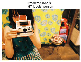
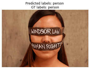
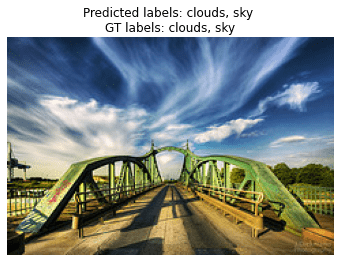
Inference example
Let’s now visually check what our network has learned to predict on images from the test set.

Summary
In this post, we’ve covered a simple yet effective approach to solving a multi-label classification problem.
The next steps would be to review more SoTA papers on the subject and try different loss functions or additional features to improve quality. For example, one of the current trends is to use GCN to provide the network with the information on which label combinations are more probable.
Subscribe & Download Code
If you liked this article and would like to download code (C++ and Python) and example images used in this post, please click here. Alternately, sign up to receive a free Computer Vision Resource Guide. In our newsletter, we share OpenCV tutorials and examples written in C++/Python, and Computer Vision and Machine Learning algorithms and news.Additional links:
For more information please refer to the following resources:
Multi-Label Text Classification
Deep dive into multi-label classification