
Back in 2012, a neural network won the ImageNet Large Scale Visual Recognition challenge for the first time. With that Alex Krizhevsky, Ilya Sutskever and Geoffrey Hinton revolutionized the area of image classification.
Nowadays, the task of assigning a single label to the image (or image classification) is well-established. However, the practical scenarios are not limited with “one label per one image” task – sometimes, we need more!
In this post, we’re going to take a look at one of the modifications of the classification task – so-called multi-output classification or image tagging.
What is multi-label classification
In the field of image classification you may encounter scenarios where you need to determine several properties of an object. For example, these can be the category, color, size, and others. In contrast with the usual image classification, the output of this task will contain 2 or more properties.
In this tutorial, we will focus on a problem where we know the number of the properties beforehand. Such task is called multi-output classification. In fact, it is a special case of multi-label classification, where you also predict several properties, but their number may vary from sample to sample.
Dataset
We will practice on the low resolution subset of the “Fashion Product Images” dataset available on Kaggle website: https://www.kaggle.com/
In this post, we’ll use Fashion Product Images dataset. It contains over 44 000 images of clothes and accessories with 9 labels for each image.
To follow the tutorial, you will need to download it and put into the folder with the code. Your folder structure should look like this:
.
├── fashion-product-images
│   ├── images
│   └── styles.csv
├── dataset.py
├── model.py
├── requirements.txt
├── split_data.py
├── test.py
└── train.py
File fashion-product-images/styles.csv contains the data labels. For the sake of simplicity, we will use only three labels in our tutorial: gender, articleType and baseColour.
Let’s take a look at some examples from the dataset:
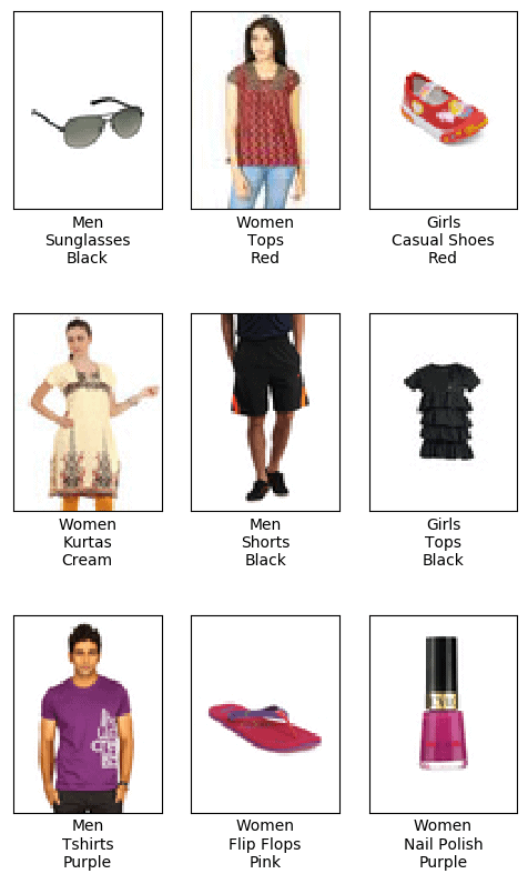
Let’s also extract all the unique labels for our categories from the data annotation. In total, we’ll have:
- 5 values for the gender (Boys, Girls, Men, Unisex, Women),
- 47 colors,
- and 143 articles (like Sports Sandals, Wallets or Sweaters).
Our goal will be to create and train a neural network model to predict three labels (gender, article, and color) for the images from our dataset.
Setup
First of all, you may want to create a new virtual python environment and install the required libraries.
Required Libraries
- matplotlib
- numpy
- pillow
- scikit-learn
- torch
- torchvision
- tqdm
All the libraries can be installed from the requirements.txt file:
python3 -m pip install -r requirements.txt
Although the code below is device-agnostic and can be run on CPU, I recommend using GPU to significantly decrease the training time. GPU is the default option in the script.
Dataset
In total, we are going to use 40 000 images. We’ll put 32 000 of them into the training set, and the rest 8 000 we’ll use for the validation. To split the data, run split_data.py script:
all_data = []
# open annotation file
with open(annotation) as csv_file:
    # parse it as CSV
    reader = csv.DictReader(csv_file)
    # tqdm shows pretty progress bar
    # each row in the CSV file corresponds to the image
    for row in tqdm(reader, total=reader.line_num):
        # we need image ID to build the path to the image file
        img_id = row['id']
        # we're going to use only 3 attributes
        gender = row['gender']
        articleType = row['articleType']
        baseColour = row['baseColour']
        img_name = os.path.join(input_folder, 'images', str(img_id) + '.jpg')
        # check if file is in place
        if os.path.exists(img_name):
            # check if the image has 80*60 pixels with 3 channels
            img = Image.open(img_name)
            if img.size == (60, 80) and img.mode == "RGB":
                all_data.append([img_name, gender, articleType, baseColour])
        else:
            print("Something went wrong: there is no file ", img_name)

# set the seed of the random numbers generator, so we can reproduce the results later
np.random.seed(42)
# construct a Numpy array from the list
all_data = np.asarray(all_data)

# Take 40000 samples in random order
inds = np.random.choice(40000, 40000, replace=False)
# split the data into train/val and save them as csv files
save_csv(all_data[inds][:32000], os.path.join(output_folder, 'train.csv'))
save_csv(all_data[inds][32000:40000], os.path.join(output_folder, 'val.csv'))
The code above creates train.csv and val.csv. These files store the list of the images and their labels in the corresponding split.
Dataset Loading
As we have more than one label in our data annotation, we need to tweak the way we read the data and load it in the memory. To do that, we’ll create a class that inherits PyTorch Dataset. It will be able to parse our data annotation and extract only the labels of our interest. The key difference between the multi-output and single-class classification is that we will return several labels per each sample from the dataset.
class FashionDataset(Dataset):
    def __init__(...):
    ...
    # initialize the arrays to store the ground truth labels and paths to the images
    self.data = []
    self.color_labels = []
    self.gender_labels = []
    self.article_labels = []

    # read the annotations from the CSV file
    with open(annotation_path) as f:
        reader = csv.DictReader(f)
        for row in reader:
            self.data.append(row['image_path'])
            self.color_labels.append(self.attr.color_name_to_id[row['baseColour']])
            self.gender_labels.append(self.attr.gender_name_to_id[row['gender']])
            self.article_labels.append(self.attr.article_name_to_id[row['articleType']])
__getitem__() function of our dataset class fetches an image and three corresponding labels. It then augments the image for the training and returns it with its labels as a dictionary:
def __getitem__(self, idx):
    # take the data sample by its index
    img_path = self.data[idx]

    # read image
    img = Image.open(img_path)

    # apply the image augmentations if needed
    if self.transform:
        img = self.transform(img)

    # return the image and all the associated labels
    dict_data = {
        'img': img,
        'labels': {
            'color_labels': self.color_labels[idx],
            'gender_labels': self.gender_labels[idx],
            'article_labels': self.article_labels[idx]
        }
    }
    return dict_data
Ok, it seems we are ready to load our data.
Data Augmentations
Data augmentations are random transformations that keep the image recognizable. They randomize the data and thus help us fight overfitting while training the network.
Here we’ll use random flipping, slight color modifications, rotation, scaling, and translation (unified in an affine transformation). We’ll also normalize the data before loading it to the network – this is a standard approach in Deep Learning.
# specify image transforms for augmentation during training
train_transform = transforms.Compose([
    transforms.RandomHorizontalFlip(p=0.5),
    transforms.ColorJitter(brightness=0.3, contrast=0.3, saturation=0.3, hue=0),
    transforms.RandomAffine(degrees=20, translate=(0.1, 0.1), scale=(0.8, 1.2),
                            shear=None, resample=False, fillcolor=(255, 255, 255)),
    transforms.ToTensor(),
    transforms.Normalize(mean, std)
])
At the validation stage, we won’t randomize the data – just normalize and convert it to PyTorch Tensor format.
# during validation we use only tensor and normalization transforms
val_transform = transforms.Compose([
    transforms.ToTensor(),
    transforms.Normalize(mean, std)
])
Now, when our dataset is ready, let’s define the model.
Model
Have a look into the model class definition. We take mobilenet_v2 network from torchvision.models. This model can solve the ImageNet classification, so its last layer is a single classifier.
To use this model for our multi-output task, we will modify it. We need to predict three properties, so we’ll use three new classification heads instead of a single classifier: these heads are called color, gender and article. Each head will have its own cross-entropy loss.
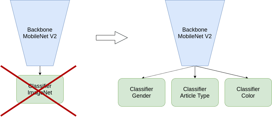
Now let’s look at how we define the network and these new heads.
class MultiOutputModel(nn.Module):
    def __init__(self, n_color_classes, n_gender_classes, n_article_classes):
        super().__init__()
        self.base_model = models.mobilenet_v2().features  # take the model without classifier
        last_channel = models.mobilenet_v2().last_channel # size of the layer before the classifier

        # the input for the classifier should be two-dimensional, but we will have
        # [<batch_size>, <channels>, <width>, <height>]
        # so, let's do the spatial averaging: reduce <width> and <height> to 1
        self.pool = nn.AdaptiveAvgPool2D((1, 1))

        # create separate classifiers for our outputs
        self.color = nn.Sequential(
            nn.Dropout(p=0.2),
            nn.Linear(in_features=last_channel, out_features=n_color_classes)
        )
        self.gender = nn.Sequential(
            nn.Dropout(p=0.2),
            nn.Linear(in_features=last_channel, out_features=n_gender_classes)
        )
        self.article = nn.Sequential(
            nn.Dropout(p=0.2),
            nn.Linear(in_features=last_channel, out_features=n_article_classes)
        )
In the forward pass through the network, we additionally average over last 2 tensor dimensions (width and height) using Adaptive Average Pooling. We do it to get a tensor suitable as an input for our classifiers. Notice we apply each classifier to the network output in parallel and return a dictionary with the three resulting values:
def forward(self, x):
    x = self.base_model(x)
    x = self.pool(x)

    # reshape from [batch, channels, 1, 1] to [batch, channels] to put it into classifier
    x = torch.flatten(x, start_dim=1)

    return {
        'color': self.color(x),
        'gender': self.gender(x),
        'article': self.article(x)
    }
Now let’s define our loss for multi-output network. In fact, we’ll just define our loss as a sum of the three losses – for color, gender and article heads:
def get_loss(self, net_output, ground_truth):
    color_loss = F.cross_entropy(net_output['color'], ground_truth['color_labels'])
    gender_loss = F.cross_entropy(net_output['gender'], ground_truth['gender_labels'])
    article_loss = F.cross_entropy(net_output['article'], ground_truth['article_labels'])
    loss = color_loss + gender_loss + article_loss
    return loss, {'color': color_loss, 'gender': gender_loss, 'article': article_loss}
Now we have both model and data ready. Let’s start the training.
Training
The training procedure for the case of multi-output classification is the same as for the single-output classification task, so I mention only several steps here. You can refer to the post on transfer learning for more details on how to code the training pipeline in PyTorch.
First, we’ll define several parameters of the training and the model itself.
Here I use small batch size as in this case it provides better accuracy. You can experiment with different values (e.g. 128 or 256) and check it yourself – the training time will decrease, but the quality may suffer.
N_epochs = 50
batch_size = 16
...

model = MultiOutputModel(n_color_classes=attributes.num_colors, n_gender_classes=attributes.num_genders,
                         n_article_classes=attributes.num_articles).to(device)

optimizer = torch.optim.Adam(model.parameters())
Then we run the training in the main loop:
for epoch in range(start_epoch, N_epochs + 1):
    ...

    for batch in train_dataloader:
        optimizer.zero_grad()
        ...
feed the data batch to the net:
        img = batch['img']
        target_labels = batch['labels']
        ...

        output = model(img.to(device))
        ...
calculate loss and accuracy:
        loss_train, losses_train = model.get_loss(output, target_labels)
        total_loss += loss_train.item()
        batch_accuracy_color, batch_accuracy_gender, batch_accuracy_article = \
           calculate_metrics(output, target_labels)
        ...
And finally, we backpropagate the error through our model and apply the resulting weight updates:
        loss_train.backward()
        optimizer.step()
        ...
Every 5 epochs we run evaluation on the validation dataset, and save the checkpoint every 25 epochs:
        if epoch % 5 == 0:
            validate(model, val_dataloader, attributes, logger, epoch, device)

        if epoch % 25 == 0:
            checkpoint_save(model, savedir, epoch)
        ...
Evaluation
Let’s return for a minute to the single-output classification task. What is the “default” metric for that problem? It’s accuracy. The definition of the accuracy in the simplest case (we do not take into account class disbalance) is the count of the correct predictions among all the data we’ve passed to the model:

What should be the metric for our multi-output classification task? Indeed, we still can use the accuracy! Recall that we have several independent outputs from the network – one per each label. We can calculate the accuracy for each label independently the same way as we did it for the single-output classification.
First, we should pass the images from the dataset to the model and get predictions. In the code below, we will do it for the “color” class, but the process is the same for all the classes that we used for the training:
# put the model into evaluation mode
model.eval()

# initialize storage for ground truth and predicted labels
predicted_color_all = []
gt_color_all = []

# go over all the images
for batch in dataloader:
    images = batch["img"]
    # we're going to build the confusion matrix for "color" predictions
    gt_colors = batch["labels"]["color_labels"]
    target_labels = {"color": gr_colors.to(device)}

    # get the model outputs
    output = model(images.to(device))

    # get the most confident prediction for each image
    _, predicted_colors = output["color"].cpu().max(1)

    predicted_color_all.extend(
        prediction.item() for prediction in predicted_colors
    )
    gt_color_all.extend(
        gt_color.item() for gt_color in gt_colors
    )
Next, with all the predictions and labels in hands, we can calculate the accuracy. To be specific, we can calculate the accuracy for each batch inside the model inference loop and average it across the batches. As we will use the predictions and ground truth values further, let’s keep them and do the accuracy computations outside the loop:
from sklearn.metrics import accuracy_score

accuracy_color = accuracy_score(gt_color_all, predicted_color_all)
If we look into the metrics, we’ll see that the final model has ~80% accuracy for the article type, 82% for the gender, and 60% for the color.
These values are good, but not great. Let’s take a look at the images and predicted labels in the test dataset:
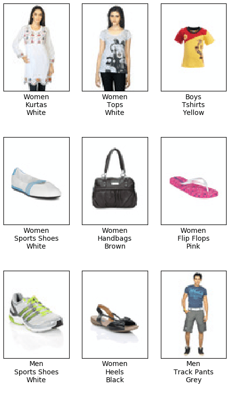
Most of the predictions look quite reasonable, so what did go wrong?
Confusion Matrix
A Confusion Matrix is a brilliant tool for debugging your image classification model. Using it, you can get valuable insights about which classes your model recognizes well and which it mixes up. Here is some theory on the confusion matrices if you need more details on how they work.
To build the confusion matrix plot, the first thing we need is the model predictions. And yes, this is why we’ve saved them earlier!
As we have predictions and ground truth labels, we’re ready to build the confusion matrix:
from sklearn.metrics import (
    confusion_matrix,
    ConfusionMatrixDisplay
)
...

cn_matrix = confusion_matrix(
    y_true=gt_color_all,
    y_pred=predicted_color_all,
    labels=attributes.color_labels,
    normalize="true",
)
ConfusionMatrixDisplay(cn_matrix, attributes.color_labels).plot(
    include_values=False, xticks_rotation="vertical"
)
plt.title("Colors")
plt.tight_layout()
plt.show()
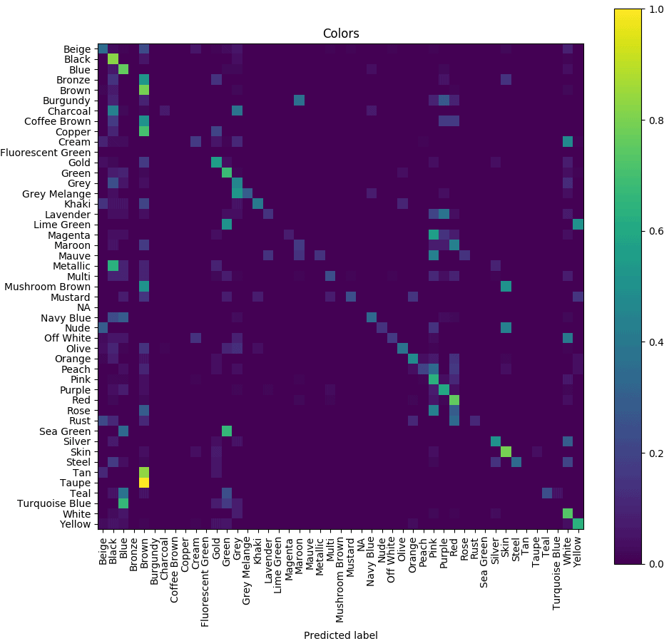
Now it’s clear that the model confuses similar colors like, for example, magenta, pink, and purple. Even for humans it would be difficult to recognize all the 47 colors represented in the dataset.
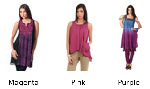
As we see, in our case, low color accuracy is not a big issue. If you want to fix it, you may decrease the number of the colors in the dataset to, for example, 10, re-mapping similar colors to one class, and then re-train the model. You should get better result.
With the gender, we see a similar behavior:
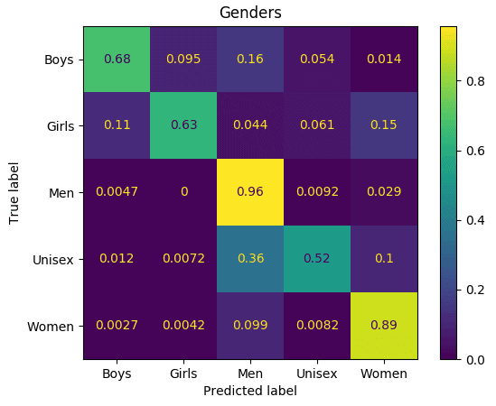
The model confuses ‘girls’ and ‘women’ labels, ‘men’ and ‘unisex’. Again, for humans, it sometimes may also be difficult to detect correct clothes labels in these cases.

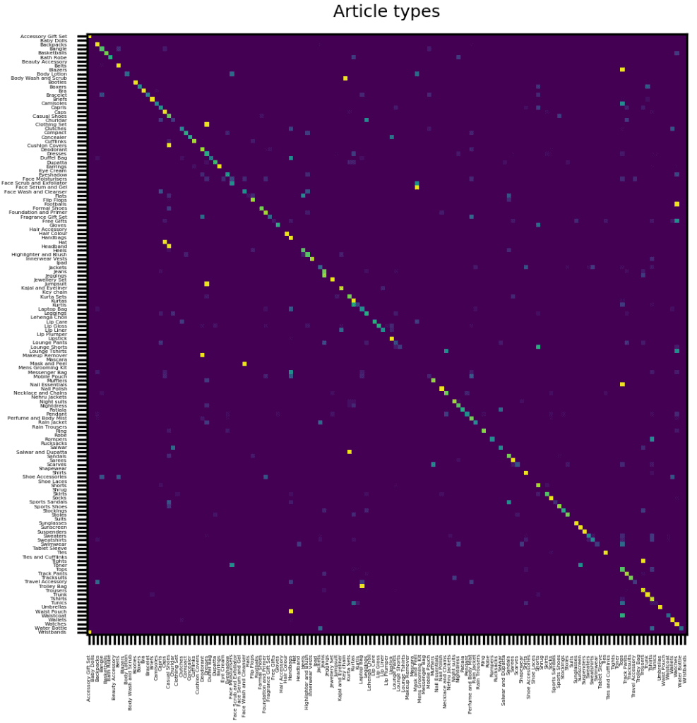
Finally, here is the confusion matrix for the clothes and accessories. Note that its main diagonal is quite distinct, that is in the most cases predicted label coincides with the ground truth:
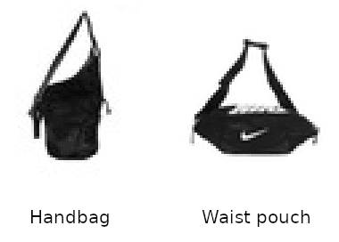
Again, some articles are just hard to distinguish – these bags below are good examples:
Summary
In this tutorial, we learned how to build a multi-output model from an existing single-output model. We also showed how to check the validity of the results using confusion matrices.
As the final advice, I recommend to always go through your dataset before the training. This way you can get a lot of insights into your data: better understand your objects of interest, the labels and their distribution in the data, and so on. This typically is a vital step to make your model achieve the top results.










100K+ Learners
Join Free OpenCV Bootcamp3 Hours of Learning