Building MobileViT from Scratch in Keras 3

In the rapidly evolving field of deep learning, the challenge often lies not just in designing powerful models but also in making them accessible and efficient for practical use, especially on devices with limited computational power. This blog post addresses this challenge by focusing on the MobileViT model, a compact yet robust alternative to the larger and more complex Vision Transformers (ViT). Our primary objective is to provide a comprehensive guide to implementing the MobileViT v1 model from scratch using Keras 3, an approach that ensures compatibility across major frameworks like TensorFlow, PyTorch, and Jax.

UPDATE June 11, 2024:
The code now works with all three backends as intended, i.e., PyTorch, TensorFlow, and JAX.

Throughout this tutorial, we will explore the intricacies of MobileViT, guiding you through the architecture and demonstrating how to code it in Keras 3. We’ll start by explaining how to port pretrained PyTorch weights into Keras 3, making it simpler for you to utilize these models without starting from zero. By converting complex PyTorch code into more readable and maintainable Keras 3 code, we aim to make advanced image classification models more accessible for deployment on resource-constrained devices such as mobile phones and edge devices.

What You’ll Gain:

By the end of this article, you will have a clear understanding of the MobileViT architecture and its advantages over traditional ViTs for deployment in constrained environments. The provided code will walk you through the different components of the MobileViT architecture and show you how to implement them effectively in Keras 3.

Bonus: Keras-Vision Python Package

To further aid your learning and implementation process, we’ve created the keras-vision Python package. This will allow you to download and experiment with the MobileViT model directly without writing any code.

By the conclusion of this post, you will be well-equipped with efficient, high-performance image classification models useful where computing power and memory are at a premium, thus broadening the reach of advanced machine learning applications.

What is Keras 3?

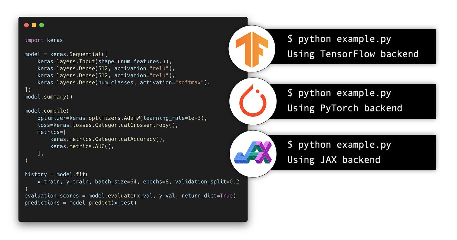
From its inception, Keras was designed as a wrapper around major frameworks such as TensorFlow and Theano (at the time). Since then, its role has undergone significant changes, and now it has returned to its original purpose: serving as a common language to facilitate communication between different frameworks and libraries, including JAX.

Keras 3 is a full rewrite of Keras that enables you to run your Keras workflows on top of either JAX, TensorFlow, or PyTorch, and that unlocks brand new large-scale model training and deployment capabilities. You can pick the framework that suits you best, and switch from one to another based on your current goals. You can also use Keras as a low-level cross-framework language to develop custom components such as layers, models, or metrics that can be used in native workflows in JAX, TensorFlow, or PyTorch — with one codebase.
— Keras 3 TeamContribution Of MobileViT

Keras 3 simplifies working across different frameworks, but that doesn’t mean you shouldn’t familiarize yourself with the underlying technologies. To truly master these tools, consider exploring our Getting Started with Keras & TensorFlow and PyTorch Series blogs.

Why MobileViT?

The Vision Transformers Landscape

Vision Transformers (ViTs) were first introduced by Dosovitskiy et al. in 2021 as an alternative to Convolutional Neural Networks (CNNs) for learning visual representations. ViTs segment an image into a sequence of non-overlapping patches and use multi-headed self-attention, a concept from the transformative 2017 paper ‘Attention is All You Need,’ to learn inter-patch representations. They can scale effectively and enhance performance as dataset sizes increase and more computational resources become available. However, these improvements come at the cost of increased parameters and latency. This need for more parameters in ViT-based models is likely due to their lack of the image-specific inductive bias inherent in CNNs.

ViTs are heavy-weight (e.g., ViT-B/16 vs. MobileNetv3: 86 vs. 7.5 million parameters), harder to optimize, need extensive data augmentation and L2 regularization to prevent over-fitting and require expensive decoders for down-stream tasks, especially for dense prediction tasks like image segmentation.

Many resource-constrained applications, such as AR and mobile deployments, still rely heavily on lightweight CNNs such as MobileNets, ESPNet’s, ShuffleNet’s, and MNASNet’s, as they are easy to optimize and integrate with task-specific networks. These networks can easily replace the heavyweight backbones like ResNet in existing task-specific models (e.g., DeepLabv3) to reduce the network size and improve latency. Despite these benefits, one major drawback of these methods is that they are spatially local.

At the time of the paper’s release, the upcoming trend (and still is, for example, FastViT) was to build robust and high-performing ViT models. So, researchers turned towards using hybrid approaches combining convolutions and transformers to get the best of both worlds. However, these hybrid models were still heavy-weight and sensitive to data augmentation. For example, removing CutMix (Zhong et al., 2020) and DeIT-style (Touvron et al., 2021a) data augmentation causes a significant drop in ImageNet accuracy (78.1% to 72.4%) of Heo et al. (2021).

It remains an open question how to combine the strengths of CNNs and transformers? to build ViT models for mobile vision tasks. Mobile vision tasks require lightweight, low latency, and accurate models that satisfy the device’s resource constraints and are general-purpose so that they can be applied to different tasks (e.g., segmentation and detection).

If you want to explore DeepLabv3 further, check out our ultimate guide to DeepLabv3 and DeepLabv3+ for a thorough exploration of this powerful segmentation model. Additionally, for those interested in leveraging the latest tools, we have a tutorial that provides practical insights and step-by-step instructions on how to use DeepLabv3+ with the new KerasCV.

Contribution Of MobileViT

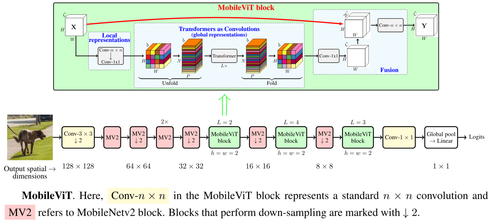
MobileViT architecture highlighting MobileViT block

The MobileViT introduces a novel approach for efficient image classification by combining the advantages of MobileNets and Vision Transformers (ViTs), their novel MobileViT-block that encodes both local and global information effectively. This hybrid architecture was designed to use the capabilities of Vision Transformers.

It basically applies “transformers as convolutions; allowing to leverage the merits of both convolutions (versatile and simple training) and transformers (global processing), which are typically more suited to larger models and datasets, to mobile and edge devices that have significant constraints on computational resources and power.

At the time of release, MobileViT punched above its weight class; it had:

Better performance: For a given parameter budget, MobileViT models achieve better performance than existing lightweight CNNs across different mobile vision tasks.
Better Generalization capability: Generalization capability measures the difference between training and evaluation metrics; MobileViT exhibits better generalization than previous ViT variants and CNNs, even outperforming them on unseen datasets despite extensive data augmentation.
More Robust: To save time and resources, a good model should be less sensitive to hyper-parameter settings like data augmentation and L2 regularization; MobileViT models can be trained effectively with basic augmentation and minimal dependence on L2 regularization.

Overall, the MobileViT model represents a significant step forward in making advanced deep learning models more accessible and practical for use in resource-constrained environments, broadening the potential applications of AI technologies in everyday devices.

Download Code To easily follow along this tutorial, please download code by clicking on the button below. It's FREE!

Click here to download the source code to this post

Building MobileViT from Scratch in Keras 3

We’ll use a bottom-up approach here. As a first step, we’ll write the required additional utility functions and common layers that are used multiple times, then (learn and) build the Transformer and the MobileViT-block. As a final step, we’ll create the entire model architecture.

Before we begin, please ensure you have either Tensorflow or PyTorch installed. Also, please update the latest keras library by executing the following:

# Install once before starting.
!pip install -U keras

Selecting Backend To Be Used

As stated, Keras 3 can support three different backends: TensorFlow, PyTorch, and Jax. As of writing this post, the provided code works as intended with TensorFlow and PyTorch and JAX backends.

But for now:

import os

# Use Either one of these as backend.
# os.environ["KERAS_BACKEND"] = "jax"
# os.environ["KERAS_BACKEND"] = "tensorflow"
os.environ["KERAS_BACKEND"] = "torch"

By default, Keras 3 looks for and uses TensorFlow as its backend. Even so, we’ve purposefully selected `torch` as it’s extraordinary to see PyTorch code not requiring standard boilerplate code.

Necessary Imports

We’ll import all the functions and classes required in the code base. The list of imports is pretty basic, as they are some of the most commonly used imports in any deep learning project.

from dataclasses import dataclass
from typing import Union, Optional

import cv2
import numpy as np
import matplotlib.pyplot as plt

import keras
import keras.ops as kops
from keras import Model, Input
from keras.layers import (
    Layer,
    Conv2D,
    DepthwiseConv2D,
    BatchNormalization,
    Activation,
    Dense,
    Dropout,
    Softmax,
    GlobalAveragePooling2D,
    LayerNormalization,
    Add,
    Identity,
    Concatenate,
    ZeroPadding2D,
)

Base Layers

In this section, we’ll define two custom Keras layers that are used in the MobileViT model. They are:

ConvLayer: It combines three layers – Conv2D, BatchNormalization, and Swish Activation.
InvertedResidualBlock: It was first introduced in the MobileNet V2 paper. We’ll describe it briefly below.

Before that, we need to define one small utility function, make_divisible(...). It basically adjusts the value v to be divisible by divisor, ensuring it does not fall below min_value and does not decrease more than 10% from v. This optimizes compatibility with hardware requirements such as GPU tensor cores.

# https://www.tensorflow.org/guide/mixed_precision#ensuring_gpu_tensor_cores_are_used
def make_divisible(v: Union[int, float], divisor: Optional[Union[int, float]] = 8, min_value: Optional[Union[int, float]] = None):
    if min_value is None:
        min_value = divisor
    new_v = max(min_value, int(v + divisor / 2) // divisor * divisor)
    # Make sure that round down does not go down by more than 10%.
    if new_v < 0.9 * v:
        new_v += divisor
    return new_v

Custom Keras 3 Layer: ConvLayer

We must remember certain caveats as we migrate from the original PyTorch codebase to Keras. The ConvLayer class is designed to facilitate the transition from PyTorch by emulating specific padding and configuration behaviors found in PyTorch’s convolutional layers.

class ConvLayer(Layer):
    def __init__(
        self,
        num_filters: int = 16,
        kernel_size: int = 3,
        strides: int = 2,
        use_activation: bool = True,
        use_bn: bool = True,
        use_bias: bool = None,
        **kwargs,
    ):
        super().__init__(**kwargs)

        self.num_filters = num_filters
        self.kernel_size = kernel_size
        self.strides = strides
        self.use_bn = use_bn
        self.use_activation = use_activation
        self.use_bias = use_bias if use_bias is not None else (False if self.use_bn else True)

        if self.strides == 2:
            self.zero_pad = ZeroPadding2D(padding=(1, 1))
            conv_padding = "valid"
        else:
            self.zero_pad = Identity()
            conv_padding = "same"
        self.conv = Conv2D(filters=self.num_filters, kernel_size=self.kernel_size, strides=self.strides, padding=conv_padding, use_bias=self.use_bias)

        if self.use_bn:
            self.bn = BatchNormalization(epsilon=1e-05, momentum=0.1)

        if self.use_activation:
            self.activation = Activation("swish")

    def call(self, x, **kwargs):
        x = self.zero_pad(x)
        x = self.conv(x)
        if self.use_bn:
            x = self.bn(x)

        if self.use_activation:
            x = self.activation(x)

        return x

    def get_config(self):
        config = super().get_config()
        config.update(
            {
                "num_filters": self.num_filters,
                "kernel_size": self.kernel_size,
                "strides": self.strides,
                "use_bias": self.use_bias,
                "use_activation": self.use_activation,
                "use_bn": self.use_bn,
            }
        )
        return config

The constructor allows for defining several key parameters such as the number of filters, kernel size, strides, and whether or not to use batch normalization (BN), an activation function, and biases.
One of the class’s convenient features is its automatic decision on the padding strategy, based on whether the stride is set to 2. This relieves you from the manual calculations and allows you to focus on other aspects of your work.
1. For stride 2, it applies zero padding (ZeroPadding2D) with padding (1, 1). It sets the convolution layer’s padding to "valid" to mimic PyTorch’s padding approach.
2. The class integrates with PyTorch for other stride values (1, 1), directly using 'same' padding in the convolution layer. This simplifies the translation process and ensures compatibility, giving you confidence in the class’s functionality.
During the forward pass (call method), the input first goes through the conditional padding mechanism, followed by the convolution operation.
If batch normalization is enabled, it is applied after the convolution along with an optional activation function, which defaults to swish.
We’ve also included the get_config(...) method, ensuring that it can be easily serialized along with custom configurations. This facilitates model saving and loading practices that are common in Keras workflows.

Custom Keras 3 Layer: InvertedResidualBlock

The Inverted Residual Block, also known as “MBConv Block”, was introduced in 2019 and is a key feature of MobileNet V2 model. MobileNet V2 was designed for efficient performance on mobile devices. It cleverly combines expansion and compression layers to ensure the model runs smoothly without consuming too much power or memory.

The inverted residual block used repetitively in MobileViT and also inside the MobileViT block.

How does an Inverted Residual Block work?

A usual residual block follows the following approach:

It has wide inputs (more channels)
The number of channels is (compressed) reduced using 1x1 (pointwise) convolutions to which a 3x3 convolution layer is applied.
The number of channels is then increased again using pointwise convolution. And if a residual connection is to be applied, the input and output are added together.

The Inverted Residual Block has an opposite approach:

It starts with a narrow input, which is then expanded using a 1x1 convolution.
Uses 3x3 Depthwise Convoltions for further feature extraction/processing.
Again, it reduces the number of channels using 1x1 convolutions.

The approach has its pros and cons. It’s efficient, fast, compact, and powerful enough for many common tasks, but it learns less complex features and might miss smaller details.

class InvertedResidualBlock(Layer):
    def __init__(
        self,
        in_channels: int = 32,
        out_channels: int = 64,
        depthwise_stride: int = 1,
        expansion_factor: Union[int, float] = 2,
        **kwargs,
    ):
        super().__init__(**kwargs)

        # Input Parameters

        self.num_in_channels = in_channels
        self.out_channels = out_channels
        self.depthwise_stride = depthwise_stride
        self.expansion_factor = expansion_factor

        num_out_channels = int(make_divisible(self.out_channels, divisor=8))
        expansion_channels = int(make_divisible(self.expansion_factor * self.num_in_channels))

        # Layer Attributes
        apply_expansion = expansion_channels > self.num_in_channels
        self.residual_connection = True if (self.num_in_channels == num_out_channels) and (self.depthwise_stride == 1) else False

        # Layers
        if apply_expansion:
            self.expansion_conv_block = ConvLayer(num_filters=expansion_channels, kernel_size=1, strides=1, use_activation=True, use_bn=True)
        else:
            self.expansion_conv_block = Identity()

        self.depthwise_conv_zero_pad = ZeroPadding2D(padding=(1, 1))
        self.depthwise_conv = DepthwiseConv2D(kernel_size=3, strides=self.depthwise_stride, padding="valid", use_bias=False)
        self.bn = BatchNormalization(epsilon=1e-05, momentum=0.1)
        self.activation = Activation("swish")
        self.out_conv_block = ConvLayer(num_filters=num_out_channels, kernel_size=1, strides=1, use_activation=False, use_bn=True)

    def call(self, data, **kwargs):
        out = self.expansion_conv_block(data)
        out = self.depthwise_conv_zero_pad(out)
        out = self.depthwise_conv(out)
        out = self.bn(out)
        out = self.activation(out)
        out = self.out_conv_block(out)

        if self.residual_connection:
            return out + data

        return out

    def get_config(self):
        config = super().get_config()
        config.update(
            {
                "in_channels": self.num_in_channels,
                "out_channels": self.out_channels,
                "depthwise_stride": self.depthwise_stride,
                "expansion_factor": self.expansion_factor,
            }
        )
        return config

Initialization: The constructor (__init__ method) sets up the block’s parameters:
1. in_channels: The number of input channels.
2. out_channels: The desired number of output channels after processing.
3. depthwise_stride: The stride used in the depthwise convolution.
4. expansion_factor: A factor by which the number of channels is expanded within the block.
Attributes:
1. The code ensures that the provided num_out_channels and calculated expansion_channels are divisible by 8, which can improve performance on certain hardware.
2. It determines whether to apply an expansion convolutional layer (apply_expansion) based on whether expansion_channels is greater than num_in_channels (input channels).
3. It sets a flag residual_connection based on conditions where a residual connection is beneficial, specifically when the input and output channels are the same and the depthwise stride is 1.
Layers:
1. If expansion is needed (apply_expansion is true), an expansion convolutional layer (expansion_conv_block) is created using the ConvLayer class. This layer increases the number of channels to expansion_channels using a 1×1 convolution.
2. The depthwise_conv_zero_pad layer applies zero padding of (1, 1) to the output of the expansion layer, preparing it for the depthwise convolution (depthwise_conv). This padding ensures that the spatial dimensions remain consistent during the depthwise convolution operation.
3. The depthwise_conv layer performs a depthwise convolution using a 3×3 kernel, the specified depthwise_stride and valid padding (no padding). This operation applies a separate convolutional filter to each input channel, reducing computational cost while capturing spatial information.
4. Batch normalization (bn) is applied after the depthwise convolution to stabilize and speed up training and passed through the Swish activation function to introduce non-linearity to the output.
5. Finally, another convolutional layer (out_conv_block) processes the output to adjust the number of output channels.
Forward Pass (call method):
1. During the forward pass, the input data is passed through the layers sequentially: expansion, padding, depthwise convolution, batch normalization, activation, and output convolution.
2. If a residual connection is enabled (residual_connection is true), the output is added to the input data before being returned.

MobileViT Block

MobileViT presents a novel approach to learning global representations by drawing inspiration from traditional convolutional layers. Traditional convolution layers are applied/processed (faster) using three key operations:

Unfolding: This step transforms both the input and the convolutional kernel into matrix forms, facilitating efficient multiplication with the input image or feature map.
Local Processing: At each spatial location, element-wise multiplication and summation are performed. This operation applies the kernel to extract local patterns and features from the input, capturing essential details.
Folding: After local processing, the results are aggregated to create the final output feature map.

operations performed when convolutions are applied

Inspired by this, the MobileViT authors:

Replace the local processing in convolutions with global processing using transformers.

This allows the MobileViT model to have CNN and ViT-like properties, which helps it learn better representations with fewer parameters and simple training recipes.

The MobileViT block consists of 3 major parts, which in turn have multiple components:

Local Representation block.
Transformers as Convolution (global representation).
Fusion.

Let’s walk through them one by one.

Local Representation Block

The "Local Representation" part of the MobileViT block.

It consists of 2 ConvLayer’s that we have previously defined.
It takes a shape $\mathbb{R}^{H \times W \times C}$ input and passes it through a (n x n) standard convolution block. Here, the kernel size is set as (3x3). This initial convolution layer encodes local spatial information within the input.
Following the initial convolution, the process continues with a pointwise convolution layer using a (1×1) kernel. This layer is designed without bias, batch normalization, or activation functions. Its primary function is to project the tensor into a higher-dimensional space by learning linear combinations of the input channels, effectively transforming the channel dimensions.

The output from this sequence of layers is a feature map of shape $\mathbb{R}^{H \times W \times d}$ , where d is greater than C, representing an expanded channel space that encapsulates both local features and broader contextual information.

Transformers as Convolution

Long-Range Dependencies: The authors aimed to capture long-range dependencies across the entire image, not just within local receptive fields. This is crucial for understanding the global context in visual data.
Challenges with Dilated Convolutions: While dilated convolutions extend the receptive field, they can inefficiently allocate weights due to the zero-padding needed to maintain image dimensions. This often results in suboptimal utilization of computational resources.
Utilizing Self-Attention: This paper’s novel approach leverages the self-attention mechanism, allowing each pixel to access information from the entire feature map. This method effectively captures global dependencies without the constraints of convolutional operations.
Spatial Inductive Bias: Traditional ViTs lack spatial inductive bias, leading to challenges in optimizability. MobileViT addresses this by introducing a method miming convolution operations through unfolding, local processing, and folding processes, which embed spatial relationships within the model architecture.
Unfolding into Non-Overlapping Patches: To enable MobileViT to learn global representations, The feature map is unfolded into N non-overlapping flattened-sized patches (h,w). The authors found that the maximum accuracy is achieved when the patch size is less than the preceding convolution kernel size (3×3) in the local representation block.

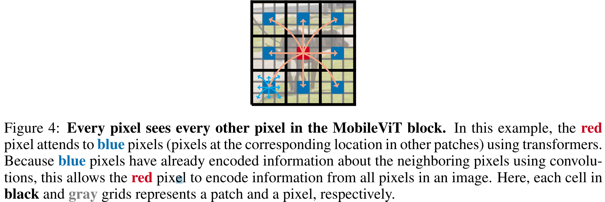
The unfolding operation used in the MobileViT block.

Global Information Exchange:
- After the unfolding operation, each patch P will only contain pixels from neighboring patches located at the same position.
- For example, referencing the above diagram, a patch will only contain pixels that are marked in blue and red.
- Because a convolution operation was applied just before, each pixel “picked” also has information about the surrounding pixels embedded in it.
- Then, to perform global processing, i.e., global exchange of information, the Transformer block is applied L times to the patches.
Folding the Output: After processing through the Transformer blocks, the output is folded back into the original image shape, maintaining the spatial structure.
Convolution-like Properties: MobileViT replaces traditional local processing in convolutions (matrix multiplication) with deeper global processing through a stack of Transformer layers, still maintaining convolution-like spatial properties.
Maintaining Spatial Order: Unlike ViTs, which can lose the spatial order of pixels, MobileViT preserves both the order of the patches and the spatial order within each patch. This is critical for maintaining coherent visual representations.
Effective Receptive Field: The effective receptive field in MobileViT covers the entire input space (H × W), allowing comprehensive contextual awareness.
Output Consistency: The output retains the same dimensional structure as the input, R^(HxWxd), facilitating easier integration with subsequent layers or operations.

Fusion

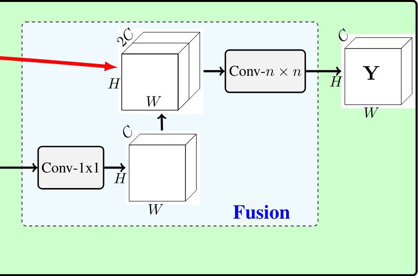
The fusion block is very simple to interpret and implement.
The input from the previous block is then projected to low C-dimensional space using a point-wise convolution and combined with the input to the MobileViT block via a concatenation operation.
Another (n × n) convolutional layer is then used to fuse these concatenated features.

MobileViT Block Code

The entire code MobileViT Block is as follows:

class MobileViT_v1_Block(Layer):
    def __init__(
        self,
        out_filters: int = 64,
        embedding_dim: int = 90,
        patch_size: Union[int, tuple] = 2,
        transformer_repeats: int = 2,
        num_heads: int = 4,
        dropout: float = 0.1,
        attention_drop: float = 0.0,
        linear_drop: float = 0.0,
        **kwargs,
    ):
        super().__init__(**kwargs)

        self.out_filters = out_filters
        self.embedding_dim = embedding_dim
        self.patch_size = patch_size
        self.transformer_repeats = transformer_repeats
        self.num_heads = num_heads
        self.dropout = dropout
        self.attention_drop = attention_drop
        self.linear_drop = linear_drop

        self.patch_size_h, self.patch_size_w = patch_size if isinstance(self.patch_size, tuple) else (self.patch_size, self.patch_size)
        self.patch_size_h, self.patch_size_w = kops.cast(self.patch_size_h, dtype="int32"), kops.cast(self.patch_size_w, dtype="int32")

        # # local_feature_extractor 1 and 2
        self.local_rep_layer_1 = ConvLayer(num_filters=self.out_filters, kernel_size=3, strides=1, use_bn=True, use_activation=True)
        self.local_rep_layer_2 = ConvLayer(num_filters=self.embedding_dim, kernel_size=1, strides=1, use_bn=False, use_activation=False, use_bias=False)

        self.transformer_layers = [
            Transformer(
                embedding_dim=self.embedding_dim,
                num_heads=self.num_heads,
                dropout=self.dropout,
                attention_drop=self.attention_drop,
                linear_drop=self.linear_drop,
            )
            for _ in range(self.transformer_repeats)
        ]

        self.transformer_layer_norm = LayerNormalization(epsilon=1e-5)

        # Fusion blocks
        self.local_features_3 = ConvLayer(num_filters=self.out_filters, kernel_size=1, strides=1, use_bn=True, use_activation=True)
        self.concat = Concatenate(axis=-1)
        self.fuse_local_global = ConvLayer(num_filters=self.out_filters, kernel_size=3, strides=1, use_bn=True, use_activation=True)

    def build(self, input_shape):
        super().build(input_shape)

    def call(self, x):

        fmH, fmW = kops.shape(x)[1], kops.shape(x)[2]

        local_representation = self.local_rep_layer_1(x)
        local_representation = self.local_rep_layer_2(local_representation)
        out_channels = local_representation.shape[-1]

        # Transformer as Convolution Steps
        # --------------------------------
        # # Unfolding

        unfolded, info_dict = self.unfolding(local_representation)

        # # Infomation sharing/mixing --> global representation
        for layer in self.transformer_layers:
            unfolded = layer(unfolded)

        global_representation = self.transformer_layer_norm(unfolded)

        # #Folding
        folded = self.folding(global_representation, info_dict=info_dict, outH=fmH, outW=fmW, outC=out_channels)

        # Fusion
        local_mix = self.local_features_3(folded)
        fusion = self.concat([x, local_mix])
        fusion = self.fuse_local_global(fusion)

        return fusion

    def get_config(self):
        config = super().get_config()
        config.update(
            {
                "out_filters": self.out_filters,
                "embedding_dim": self.embedding_dim,
                "patch_size": self.patch_size,
                "transformer_repeats": self.transformer_repeats,
                "num_heads": self.num_heads,
                "dropout": self.dropout,
                "attention_drop": self.attention_drop,
                "linear_drop": self.linear_drop,
            }
        )
        return config

The unfolding(...) and folding(...) methods are part of the MobileViT block class and are 1:1 replicated from the original pytorch codebase. There are some optimizations that can be done to improve the speed. We’ll update this section as well.

    def unfolding(self, feature_map):
        # Initially convert channel-last to channel-first for processing
        shape = kops.shape(feature_map)
        batch_size, orig_h, orig_w, in_channels = shape[0], shape[1], shape[2], shape[3]
        feature_map = kops.transpose(feature_map, [0, 3, 1, 2])  # [B, H, W, C] -> [B, C, H, W]

        patch_area = self.patch_size_w * self.patch_size_h

        orig_h, orig_w = kops.cast(orig_h, dtype="int32"), kops.cast(orig_w, dtype="int32")

        h_ceil = kops.ceil(orig_h / self.patch_size_h)
        w_ceil = kops.ceil(orig_w / self.patch_size_w)

        new_h = kops.cast(h_ceil * kops.cast(self.patch_size_h, dtype=h_ceil.dtype), dtype="int32")
        new_w = kops.cast(w_ceil * kops.cast(self.patch_size_w, dtype=h_ceil.dtype), dtype="int32")

        # Condition to decide if resizing is necessary
        resize_required = kops.logical_or(kops.not_equal(new_w, orig_w), kops.not_equal(new_h, orig_h))
        feature_map = kops.cond(
            resize_required,
            true_fn=lambda: kops.image.resize(feature_map, [new_h, new_w], data_format="channels_first"),
            false_fn=lambda: feature_map,
        )

        num_patch_h = new_h // self.patch_size_h
        num_patch_w = new_w // self.patch_size_w
        num_patches = num_patch_h * num_patch_w

        # Handle dynamic shape multiplication
        dynamic_shape_mul = kops.prod([batch_size, in_channels * num_patch_h])

        # Reshape and transpose to create patches
        reshaped_fm = kops.reshape(feature_map, [dynamic_shape_mul, self.patch_size_h, num_patch_w, self.patch_size_w])
        transposed_fm = kops.transpose(reshaped_fm, [0, 2, 1, 3])
        reshaped_fm = kops.reshape(transposed_fm, [batch_size, in_channels, num_patches, patch_area])
        transposed_fm = kops.transpose(reshaped_fm, [0, 3, 2, 1])
        patches = kops.reshape(transposed_fm, [batch_size * patch_area, num_patches, in_channels])

        info_dict = {
            "orig_size": (orig_h, orig_w),
            "batch_size": batch_size,
            "interpolate": resize_required,
            "total_patches": num_patches,
            "num_patches_w": num_patch_w,
            "num_patches_h": num_patch_h,
            "patch_area": patch_area,
        }

        return patches, info_dict

    def folding(self, patches, info_dict, outH, outW, outC):
        # Ensure the input patches tensor has the correct dimensions
        assert len(patches.shape) == 3, f"Tensor should be of shape BPxNxC. Got: {patches.shape}"

        # Reshape to [B, P, N, C]
        patches = kops.reshape(patches, [info_dict["batch_size"], info_dict["patch_area"], info_dict["total_patches"], -1])

        # Get shape parameters for further processing
        shape = kops.shape(patches)
        batch_size = shape[0]
        channels = shape[3]

        num_patch_h = info_dict["num_patches_h"]
        num_patch_w = info_dict["num_patches_w"]

        # Transpose dimensions [B, P, N, C] --> [B, C, N, P]
        patches = kops.transpose(patches, [0, 3, 2, 1])

        # Calculate total elements dynamically
        num_total_elements = batch_size * channels * num_patch_h

        # Reshape to match the size of the feature map before splitting into patches
        # [B, C, N, P] --> [B*C*n_h, n_w, p_h, p_w]
        feature_map = kops.reshape(patches, [num_total_elements, num_patch_w, self.patch_size_h, self.patch_size_w])

        # Transpose to switch width and height axes [B*C*n_h, n_w, p_h, p_w] --> [B*C*n_h, p_h, n_w, p_w]
        feature_map = kops.transpose(feature_map, [0, 2, 1, 3])

        # Reshape back to the original image dimensions [B*C*n_h, p_h, n_w, p_w] --> [B, C, H, W]
        # Reshape back to [B, C, H, W]
        new_height = num_patch_h * self.patch_size_h
        new_width = num_patch_w * self.patch_size_w
        feature_map = kops.reshape(feature_map, [batch_size, -1, new_height, new_width])

        # Conditional resizing using kops.cond
        feature_map = kops.cond(
            info_dict["interpolate"],
            lambda: kops.image.resize(feature_map, info_dict["orig_size"], data_format="channels_first"),
            lambda: feature_map,
        )

        feature_map = kops.transpose(feature_map, [0, 2, 3, 1])
        feature_map = kops.reshape(feature_map, (batch_size, outH, outW, outC))

        return feature_map

To complete the MobileViT Block, two more additional layers are required:

Multi-head self-attention (MHSA).
Transformer layer.

Multi-Head Self-Attention Block

Let’s implement the MHSA layer first.

class MHSA(Layer):
    def __init__(
        self,
        num_heads: int = 2,
        embedding_dim: int = 64,
        projection_dim: int = None,
        qkv_bias: bool = True,
        attention_drop: float = 0.2,
        linear_drop: float = 0.2,
    ):
        super().__init__()
        self.num_heads = num_heads
        self.embedding_dim = embedding_dim
        self.projection_dim = projection_dim if projection_dim else embedding_dim // num_heads
        self.qkv_bias = qkv_bias
        self.scale = self.projection_dim**-0.5

        self.qkv = Dense(3 * self.num_heads * self.projection_dim, use_bias=qkv_bias)
        self.proj = Dense(embedding_dim, use_bias=qkv_bias)
        self.attn_dropout = Dropout(attention_drop)
        self.linear_dropout = Dropout(linear_drop)
        self.softmax = Softmax()

    def build(self, input_shape):
        # You can perform setup tasks that depend on the input shape here
        super().build(input_shape)

    def split_heads(self, x, batch_size):
        # Split the last dimension into (num_heads, projection_dim)
        x = kops.reshape(x, (batch_size, -1, self.num_heads, self.projection_dim))
        # Transpose to shape (batch_size, num_heads, seq_len, projection_dim)
        return kops.transpose(x, axes=(0, 2, 1, 3))

    def call(self, x):
        batch_size = kops.shape(x)[0]

        # Project and reshape to (batch_size, seq_len, 3, num_heads, projection_dim)
        qkv = self.qkv(x)
        qkv = kops.reshape(qkv, (batch_size, -1, 3, self.num_heads, self.projection_dim))
        qkv = kops.transpose(qkv, axes=(0, 2, 1, 3, 4))
        q, k, v = qkv[:, 0], qkv[:, 1], qkv[:, 2]

        q = self.split_heads(q, batch_size)
        k = self.split_heads(k, batch_size)
        v = self.split_heads(v, batch_size)

        q *= self.scale

        # Attention mechanism
        attn_logits = kops.matmul(q, kops.transpose(k, axes=(0, 1, 3, 2)))
        attn = self.softmax(attn_logits)
        attn = self.attn_dropout(attn)

        weighted_avg = kops.matmul(attn, v)
        weighted_avg = kops.transpose(weighted_avg, axes=(0, 2, 1, 3))
        weighted_avg = kops.reshape(weighted_avg, (batch_size, -1, self.num_heads * self.projection_dim))

        # Output projection
        output = self.proj(weighted_avg)
        output = self.linear_dropout(output)

        return output

Custom Transformer Block

This layer is encompassed by a LayerNormalization, followed by Dropout and Dense layers. Together, these components constitute the Transformer layer.

class Transformer(Layer):
    def __init__(
        self,
        num_heads: int = 4,
        embedding_dim: int = 90,
        qkv_bias: bool = True,
        mlp_ratio: float = 2.0,
        dropout: float = 0.1,
        linear_drop: float = 0.0,
        attention_drop: float = 0.0,
        **kwargs,
    ):
        super().__init__(**kwargs)
        self.num_heads = num_heads
        self.embedding_dim = embedding_dim
        self.qkv_bias = qkv_bias
        self.mlp_ratio = mlp_ratio
        self.dropout = dropout
        self.linear_drop = linear_drop
        self.attention_drop = attention_drop

        self.norm_1 = LayerNormalization(epsilon=1e-5)

        self.attn = MHSA(
            num_heads=self.num_heads,
            embedding_dim=self.embedding_dim,
            qkv_bias=self.qkv_bias,
            attention_drop=self.attention_drop,
            linear_drop=dropout,
        )
        self.norm_2 = LayerNormalization(epsilon=1e-5)

        hidden_features = int(self.embedding_dim * self.mlp_ratio)

        self.mlp_block_0 = Dense(hidden_features, activation="swish")
        self.mlp_block_1 = Dropout(self.linear_drop)
        self.mlp_block_2 = Dense(embedding_dim)
        self.mlp_block_3 = Dropout(dropout)

    def build(self, input_shape):
        super().build(input_shape)

    def call(self, x):
        x = x + self.attn(self.norm_1(x))

        mlp_block_out = self.mlp_block_0(self.norm_2(x))
        mlp_block_out = self.mlp_block_1(mlp_block_out)
        mlp_block_out = self.mlp_block_2(mlp_block_out)
        mlp_block_out = self.mlp_block_3(mlp_block_out)

        x = x + mlp_block_out

        return x

    def get_config(self):
        config = super().get_config()
        config.update(
            {
                "num_heads": self.num_heads,
                "embedding_dim": self.embedding_dim,
                "qkv_bias": self.qkv_bias,
                "mlp_ratio": self.mlp_ratio,
                "dropout": self.dropout,
                "linear_drop": self.linear_drop,
                "attention_drop": self.attention_drop,
            }
        )
        return config

Building MobileViT Architecture

The architecture table detailing MobileViT model variants.

Inspiration from Lightweight CNNs: MobileViT draws inspiration from the design philosophy of lightweight CNNs, which aim to maximize efficiency and minimize computational overhead.
Architecture Overview: The MobileViT architecture begins with a strided 3x3 standard convolution layer, followed by MobileNet v2 blocks and MobileViT blocks
Simplified Design with Variants: The authors have streamlined the architecture to keep it simple while offering three variants—XXS, XS, and S—with parameters ranging from 1.3 million to 5.6 million, catering to different computational capacities and application needs.
Role of MobileNet Blocks: The MobileNet blocks primarily handle down-sampling tasks within the model. They utilize an expansion factor of four, although for the MobileViT-XXS variant, a reduced expansion factor of two is used to adapt to more constrained environments.
Activation Function: Throughout the architecture, the Swish activation function introduces non-linearity, enhancing the model’s ability to learn complex patterns.
Kernel and Patch Sizes: Within the MobileViT blocks, the authors employ 3x3 convolutional kernels and 2x2 patch sizes, balancing local processing and global contextual understanding.

As we have defined all the required custom layers, putting together the entire model architecture is quite straightforward by referencing the above architecture table:

def MobileViT_v1(
    configs,
    dropout: float = 0.1,
    linear_drop: float = 0.0,
    attention_drop: float = 0.0,
    num_classes: int | None = 1000,
    input_shape: tuple[int, int, int] = (256, 256, 3),
    model_name: str = f"MobileViT_v1-S",
):
    """
    Arguments
    --------

        configs: A dataclass instance with model information such as per layer output channels, transformer embedding dimensions, transformer repeats, IR expansion factor

        num_classes: (int)   Number of output classes

        input_shape: (tuple) Input shape -> H, W, C

        model_type: (str)   Model to create

        linear_drop: (float) Dropout rate for Dense layers

        attention_drop: (float) Dropout rate for the attention matrix

    """

    input_layer = Input(shape=input_shape)

    # Block 1
    out = ConvLayer(
        num_filters=configs.block_1_1_dims,
        kernel_size=3,
        strides=2,
        name="block-1-Conv",
    )(input_layer)

    out = InvertedResidualBlock(
        in_channels=configs.block_1_1_dims,
        out_channels=configs.block_1_2_dims,
        depthwise_stride=1,
        expansion_factor=configs.depthwise_expansion_factor,
        name="block-1-IR2",
    )(out)

    # Block 2
    out = InvertedResidualBlock(
        in_channels=configs.block_1_2_dims,
        out_channels=configs.block_2_1_dims,
        depthwise_stride=2,
        expansion_factor=configs.depthwise_expansion_factor,
        name="block-2-IR1",
    )(out)

    out = InvertedResidualBlock(
        in_channels=configs.block_2_1_dims,
        out_channels=configs.block_2_2_dims,
        depthwise_stride=1,
        expansion_factor=configs.depthwise_expansion_factor,
        name="block-2-IR2",
    )(out)

    out = InvertedResidualBlock(
        in_channels=configs.block_2_2_dims,
        out_channels=configs.block_2_3_dims,
        depthwise_stride=1,
        expansion_factor=configs.depthwise_expansion_factor,
        name="block-2-IR3",
    )(out)

    # Block 3
    out = InvertedResidualBlock(
        in_channels=configs.block_2_2_dims,
        out_channels=configs.block_3_1_dims,
        depthwise_stride=2,
        expansion_factor=configs.depthwise_expansion_factor,
        name="block-3-IR1",
    )(out)

    out = MobileViT_v1_Block(
        out_filters=configs.block_3_2_dims,
        embedding_dim=configs.tf_block_3_dims,
        transformer_repeats=configs.tf_block_3_repeats,
        name="MobileViTBlock-1",
        dropout=dropout,
        attention_drop=attention_drop,
        linear_drop=linear_drop,
    )(out)

    # Block 4
    out = InvertedResidualBlock(
        in_channels=configs.block_3_2_dims,
        out_channels=configs.block_4_1_dims,
        depthwise_stride=2,
        expansion_factor=configs.depthwise_expansion_factor,
        name="block-4-IR1",
    )(out)

    out = MobileViT_v1_Block(
        out_filters=configs.block_4_2_dims,
        embedding_dim=configs.tf_block_4_dims,
        transformer_repeats=configs.tf_block_4_repeats,
        name="MobileViTBlock-2",
        dropout=dropout,
        attention_drop=attention_drop,
        linear_drop=linear_drop,
    )(out)

    # Block 5
    out = InvertedResidualBlock(
        in_channels=configs.block_4_2_dims,
        out_channels=configs.block_5_1_dims,
        depthwise_stride=2,
        expansion_factor=configs.depthwise_expansion_factor,
        name="block-5-IR1",
    )(out)

    out = MobileViT_v1_Block(
        out_filters=configs.block_5_2_dims,
        embedding_dim=configs.tf_block_5_dims,
        transformer_repeats=configs.tf_block_5_repeats,
        name="MobileViTBlock-3",
        dropout=dropout,
        attention_drop=attention_drop,
        linear_drop=linear_drop,
    )(out)

    out = ConvLayer(num_filters=configs.final_conv_dims, kernel_size=1, strides=1, name="final_conv")(out)

    if num_classes:
        # Output layer
        out = GlobalAveragePooling2D()(out)

        if linear_drop > 0.0:
            out = Dropout(rate=dropout)(out)

        out = Dense(units=num_classes)(out)

    model = Model(inputs=input_layer, outputs=out, name=model_name)

    return model

MobileViT Model Configurations

We’ve created a configuration class for each variant so that you can quickly load and change it.

For instance, let’s take a look at the configuration of the MobileVIT-S model, a prime example of how our model configurations can be defined:

@dataclass
class Config_MobileViT_v1_S:
    block_1_1_dims: int = 16
    block_1_2_dims: int = 32

    block_2_1_dims: int = 64
    block_2_2_dims: int = 64
    block_2_3_dims: int = 64

    block_3_1_dims: int = 96
    block_3_2_dims: int = 96

    block_4_1_dims: int = 128
    block_4_2_dims: int = 128

    block_5_1_dims: int = 160
    block_5_2_dims: int = 160

    final_conv_dims: int = 640

    tf_block_3_dims: int = 144
    tf_block_4_dims: int = 192
    tf_block_5_dims: int = 240

    tf_block_3_repeats: int = 2
    tf_block_4_repeats: int = 4
    tf_block_5_repeats: int = 3

    depthwise_expansion_factor: int = 4

And here’s the helper function to load these configs:

def build_MobileViT_v1(
    model_type: str = "S",
    num_classes: int = 1000,
    input_shape: tuple = (256, 256, 3),
    include_top: bool = True,  # Whether to include the classification layer in the model
    updates: Optional[dict] = None,
    **kwargs,
):
    """
    Create MobileViT-v1 Classification models or feature extractors with optional pretrained weights.

    Arguments:
    ---------
        model_type: (str)   MobileViT version to create. Options: S, XS, XXS
        num_classes: (int)   Number of output classes
        input_shape: (tuple) Input shape -> H, W, C
        include_top: (bool) Whether to include the classification layers
        updates: (dict) a key-value pair indicating the changes to be made to the base model.

    Additional arguments:
    ---------------------
        linear_drop: (float) Dropout rate for Dense layers
        attention_drop: (float) Dropout rate for the attention matrix
    """
    model_type = model_type.upper()
    if model_type not in ("S", "XS", "XXS"):
        raise ValueError("Bad Input. 'model_type' should be one of ['S', 'XS', 'XXS']")

    updated_configs = get_mobile_vit_v1_configs(model_type, updates=updates)

    # Build the base model
    model = MobileViT_v1(
        configs=updated_configs,
        num_classes=num_classes if include_top else None,
        input_shape=input_shape,
        model_name=f"MobileViT_v1-{model_type}",
        **kwargs,
    )

    return model

As a result, we can simply do the following:

model = build_MobileViT_v1(
    model_type="XXS",  # "XS", "XXS"
    input_shape=(256, 256, 3),  # (None, None, 3)
    num_classes=1000,
    linear_drop=0.0,
    attention_drop=0.0,
    dropout=0.1,
)
model.summary()

Model: "MobileViT_v1-S"
┏━━━━━━━━━━━━━━━━━━━━━━━━━━━━━━━━━━━━━━┳━━━━━━━━━━━━━━━━━━━━━━━━━━━━━┳━━━━━━━━━━━━━━━━━┓
┃ Layer (type)                         ┃ Output Shape                ┃         Param # ┃
┡━━━━━━━━━━━━━━━━━━━━━━━━━━━━━━━━━━━━━━╇━━━━━━━━━━━━━━━━━━━━━━━━━━━━━╇━━━━━━━━━━━━━━━━━┩
│ input_layer (InputLayer)             │ (None, 256, 256, 3)         │               0 │
├──────────────────────────────────────┼─────────────────────────────┼─────────────────┤
│ block-1-Conv (ConvLayer)             │ (None, 128, 128, 16)        │             496 │
├──────────────────────────────────────┼─────────────────────────────┼─────────────────┤
│ block-1-IR2 (InvertedResidualBlock)  │ (None, 128, 128, 32)        │           4,288 │
├──────────────────────────────────────┼─────────────────────────────┼─────────────────┤
│ block-2-IR1 (InvertedResidualBlock)  │ (None, 64, 64, 64)          │          14,720 │
├──────────────────────────────────────┼─────────────────────────────┼─────────────────┤
│ block-2-IR2 (InvertedResidualBlock)  │ (None, 64, 64, 64)          │          37,376 │
├──────────────────────────────────────┼─────────────────────────────┼─────────────────┤
│ block-2-IR3 (InvertedResidualBlock)  │ (None, 64, 64, 64)          │          37,376 │
├──────────────────────────────────────┼─────────────────────────────┼─────────────────┤
│ block-3-IR1 (InvertedResidualBlock)  │ (None, 32, 32, 96)          │          45,696 │
├──────────────────────────────────────┼─────────────────────────────┼─────────────────┤
│ MobileViTBlock-1                     │ (None, 32, 32, 96)          │         612,864 │
│ (MobileViT_v1_Block)                 │                             │                 │
├──────────────────────────────────────┼─────────────────────────────┼─────────────────┤
│ block-4-IR1 (InvertedResidualBlock)  │ (None, 16, 16, 128)         │          93,056 │
├──────────────────────────────────────┼─────────────────────────────┼─────────────────┤
│ MobileViTBlock-2                     │ (None, 16, 16, 128)         │       1,681,536 │
│ (MobileViT_v1_Block)                 │                             │                 │
├──────────────────────────────────────┼─────────────────────────────┼─────────────────┤
│ block-5-IR1 (InvertedResidualBlock)  │ (None, 8, 8, 160)           │         156,800 │
├──────────────────────────────────────┼─────────────────────────────┼─────────────────┤
│ MobileViTBlock-3                     │ (None, 8, 8, 160)           │       2,160,720 │
│ (MobileViT_v1_Block)                 │                             │                 │
├──────────────────────────────────────┼─────────────────────────────┼─────────────────┤
│ conv_layer_26 (ConvLayer)            │ (None, 8, 8, 640)           │         104,960 │
├──────────────────────────────────────┼─────────────────────────────┼─────────────────┤
│ global_average_pooling2d             │ (None, 640)                 │               0 │
│ (GlobalAveragePooling2D)             │                             │                 │
├──────────────────────────────────────┼─────────────────────────────┼─────────────────┤
│ dense_36 (Dense)                     │ (None, 1000)                │         641,000 │
└──────────────────────────────────────┴─────────────────────────────┴─────────────────┘
 Total params: 5,590,888 (21.33 MB)
 Trainable params: 5,578,632 (21.28 MB)
 Non-trainable params: 12,256 (47.88 KB)

We can customize any setting by creating a dictionary of the configurations we want to change:

# Refer to BaseConfigs class to see all customizable modules available.
updates = {
    "block_3_1_dims": 96,
    "block_3_2_dims": 96,
    "tf_block_3_dims": 164,
    "tf_block_3_repeats": 2,
}

model = build_MobileViT_v1(
    model_type="S",
    updates=updates,
)

print(f"{model.name} num. parameters: {model.count_params()}")

MobileViT_v1-S num. parametes: 5693768

Model: "MobileViT_v1-S"
┏━━━━━━━━━━━━━━━━━━━━━━━━━━━━━━━━━━━━━┳━━━━━━━━━━━━━━━━━━━━━━━━━━━━━━━━━━┳━━━━━━━━━━━━━┓
┃ Layer (type)                        ┃ Output Shape                     ┃     Param # ┃
┡━━━━━━━━━━━━━━━━━━━━━━━━━━━━━━━━━━━━━╇━━━━━━━━━━━━━━━━━━━━━━━━━━━━━━━━━━╇━━━━━━━━━━━━━┩
│ input_layer_1 (InputLayer)          │ (None, 256, 256, 3)              │           0 │
├─────────────────────────────────────┼──────────────────────────────────┼─────────────┤
│ block-1-Conv (ConvLayer)            │ (None, 128, 128, 16)             │         496 │
├─────────────────────────────────────┼──────────────────────────────────┼─────────────┤
│ block-1-IR2 (InvertedResidualBlock) │ (None, 128, 128, 32)             │       4,288 │
├─────────────────────────────────────┼──────────────────────────────────┼─────────────┤
│ block-2-IR1 (InvertedResidualBlock) │ (None, 64, 64, 64)               │      14,720 │
├─────────────────────────────────────┼──────────────────────────────────┼─────────────┤
│ block-2-IR2 (InvertedResidualBlock) │ (None, 64, 64, 64)               │      37,376 │
├─────────────────────────────────────┼──────────────────────────────────┼─────────────┤
│ block-2-IR3 (InvertedResidualBlock) │ (None, 64, 64, 64)               │      37,376 │
├─────────────────────────────────────┼──────────────────────────────────┼─────────────┤
│ block-3-IR1 (InvertedResidualBlock) │ (None, 32, 32, 96)               │      45,696 │
├─────────────────────────────────────┼──────────────────────────────────┼─────────────┤
│ MobileViTBlock-1                    │ (None, 32, 32, 96)               │     715,744 │
│ (MobileViT_v1_Block)                │                                  │             │
├─────────────────────────────────────┼──────────────────────────────────┼─────────────┤
│ block-4-IR1 (InvertedResidualBlock) │ (None, 16, 16, 128)              │      93,056 │
├─────────────────────────────────────┼──────────────────────────────────┼─────────────┤
│ MobileViTBlock-2                    │ (None, 16, 16, 128)              │   1,681,536 │
│ (MobileViT_v1_Block)                │                                  │             │
├─────────────────────────────────────┼──────────────────────────────────┼─────────────┤
│ block-5-IR1 (InvertedResidualBlock) │ (None, 8, 8, 160)                │     156,800 │
├─────────────────────────────────────┼──────────────────────────────────┼─────────────┤
│ MobileViTBlock-3                    │ (None, 8, 8, 160)                │   2,160,720 │
│ (MobileViT_v1_Block)                │                                  │             │
├─────────────────────────────────────┼──────────────────────────────────┼─────────────┤
│ conv_layer_53 (ConvLayer)           │ (None, 8, 8, 640)                │     104,960 │
├─────────────────────────────────────┼──────────────────────────────────┼─────────────┤
│ global_average_pooling2d_1          │ (None, 640)                      │           0 │
│ (GlobalAveragePooling2D)            │                                  │             │
├─────────────────────────────────────┼──────────────────────────────────┼─────────────┤
│ dense_73 (Dense)                    │ (None, 1000)                     │     641,000 │
└─────────────────────────────────────┴──────────────────────────────────┴─────────────┘
 Total params: 5,693,768 (21.72 MB)
 Trainable params: 5,681,512 (21.67 MB)
 Non-trainable params: 12,256 (47.88 KB)

Porting PyTorch Weights to Keras 3

In this section, we will explain how to port weights from PyTorch to Keras. By default, PyTorch’s state_dict saves weights in a channel_first format, whereas TensorFlow as well as Keras follows a channels_last format. Therefore, we need to keep these differences in mind during the porting process. As we have replicated the original PyTorch codebase, we don’t have to worry about mismatches between layers and their weights shape at any point. We can simply iterate through the Keras 3 and PyTorch model weights.

In our use case, we need to be aware of three main differences:

Dense Layers:
1. In Keras, the Dense layer weights are stored in (in_features, out_features) manner.
2. Whereas in PyTorch, the Linear layer weights are stored in (out_features, in_features) format.
3. So when we iterate over the PyTorch weights, we’ll have to transpose them to match the required Keras weights shape.
Convolution layers:
1. The kernel weights are stored in format (kH, kW, inC, outC) in Keras.
2. In PyTorch, the kernel weights are stored in (outC, inC, kH, kW) format.
3. To match the shapes, we’ll have to permute the PyTorch weights as follows: param.permute(2, 3, 1, 0).
Depthwise Convolution layers:
1. In Keras, we have a separate layer to perform Depthwise convolutions, which stores the kernel in format (kH, kW, outC, inC).
2. In contrast, in PyTorch, there’s no separate layer to perform Depthwise convolutions; it is done by passing groups=inC, so the kernels are stored in the same format as Convolution layers.
3. To match PyTorch and Keras kernel shape, we have to perform a permute operation as follows: param.permute(2, 3, 0, 1)

To facilitate the process, we have defined a WeightsLayerIterator class and two helper functions: get_pytorch2keras_layer_weights_mapping(...) and load_weights_in_keras_model(...).

WeightsLayerIterator class: Apart from taking care of the transpose and permute operations as explained above, we also need to skip some key-value pairs in PyTorch and Keras as they don’t have any parameters. For, e.g. the num_batches_tracked variable of the BatchNormalization layer in PyTorch and seed_generator_state in Keras.

class WeightsLayerIterator:
    def __init__(self, pytorch_weights, keras_model):
        self.keras_model = keras_model
        self.pytorch_weights = pytorch_weights
        self.keras_layer_is_depthwise = False
        self.keras_layer_is_einsum = False

    def get_next_pytorch_weight(self):
        count = 0
        for idx, (param_name, param) in enumerate(self.pytorch_weights.items()):

            sentence = "{count} {param_name} ----> {param_shape}"
            if "num_batches_tracked" in param_name:
                continue
            if "conv.weight" in param_name:
                if self.keras_layer_is_depthwise:
                    param = param.permute(2, 3, 0, 1)
                else:
                    param = param.permute(2, 3, 1, 0)

            elif len(param.shape) == 2:
                param = param.T
            count += 1
            yield sentence.format(count=count, param_name=param_name, param_shape=param.shape), param

    def get_keras_weight(self):
        count = 0
        for idx, param in enumerate(self.keras_model.variables):
            if "seed_generator_state" in param.path:
                continue

            self.keras_layer_is_depthwise = True if "depthwise_conv2d" in param.path else False

            count += 1
            yield f"{count} {param.path} ----> {param.shape}", param

The get_pytorch2keras_layer_weights_mapping(...) is designed to help create a dictionary map between Keras layers and weights in PyTorch corresponding to that layer. For each weight pair, it extracts the Keras layer name from the weight path and stores all the PyTorch weight’s as a list.

def get_pytorch2keras_layer_weights_mapping(pytorch_weights, keras_model):
    wl = WeightsLayerIterator(pytorch_weights=pytorch_weights, keras_model=keras_model)
    layer_mapping = {}
    for (keras_sentence, keras_weight), (pytorch_sentence, pytorch_weight) in zip(wl.get_keras_weight(), wl.get_next_pytorch_weight()):
        keras_layer_name = keras_weight.path.split("/")[0]
        layer_mapping.setdefault(keras_layer_name, list())
        layer_mapping[keras_layer_name].append(pytorch_weight.numpy())

    return layer_mapping

Download pretrained weights:

!wget -qnc https://docs-assets.developer.apple.com/ml-research/models/cvnets/classification/mobilevit_s.pt -O mobilevit_s.pt

Load PyTorch weights and Keras model:

import torch

pytorch_weights_s = torch.load("mobilevit_s.pt", map_location="CPU")

keras_model_S = build_MobileViT_v1(model_type="S", input_shape=(256, 256, 3))

Then, we can do:

keras_model_s_layer_mapping   = get_pytorch2keras_layer_weights_mapping(pytorch_weights=pytorch_weights_s, keras_model=keras_model_S)

Then all there’s left is to iterate over each layer in Keras and use the set_weight operation to overwrite the current weights.

def load_weights_in_keras_model(keras_model, layer_mapping):
    for keras_layer in keras_model.layers[1:]:
        keras_layer_name = keras_layer.name

        if "global_average_pooling2d" in keras_layer_name:
            continue

        if "dropout" in keras_layer.name:
            continue

        from_pt = list(layer_mapping[keras_layer_name])
        keras_model.get_layer(keras_layer_name).set_weights(from_pt)
    return keras_model

keras_model_S = load_weights_in_keras_model(keras_model=keras_model_S, layer_mapping=keras_model_s_layer_mapping)

And that’s it.

We can now test the model’s prediction using random classes from Imagenet-1k classes to verify if the pretrained weights are loaded and if the layer-wise operation performed is working correctly. To do so, we’ll write one final helper function to test the model.

def test_prediction(*, image_path, model, show=False):
    # Load and process the image
    img = cv2.imread(image_path, cv2.IMREAD_COLOR) # NOT CONVERTED to RGB (required).

    img = cv2.resize(img, (256, 256))  # Resize image to match model's expected input

    if show:
        plt.imshow(img[:, :, ::-1])
        plt.axis("off")
        plt.show()

    img = img  / 255. # Normalize pixel values to [0, 1]
    img = img.astype("float32")  # Ensure the correct type for TensorFlow
    # Add the batch dimension
    img_tf = np.expand_dims(img, 0)  # Shape becomes (1, 256, 256, 3)

    # Perform prediction
    preds = model.predict(img_tf, verbose=0)

    # Output prediction
    print(f"Model: {model.name}, Predictions: {preds.argmax()}")

Let’s download a cat and panda image from Wikipedia first:

!wget -qnc https://upload.wikimedia.org/wikipedia/commons/thumb/6/68/Orange_tabby_cat_sitting_on_fallen_leaves-Hisashi-01A.jpg/1024px-Orange_tabby_cat_sitting_on_fallen_leaves-Hisashi-01A.jpg -O cat.jpg

!wget -qnc https://upload.wikimedia.org/wikipedia/commons/thumb/0/0f/Grosser_Panda.JPG/1920px-Grosser_Panda.JPG -O pandas.jpg

Test:

test_prediction(image_path="cat.jpg", model=keras_model_XXS, show=True)
test_prediction(image_path="pandas.jpg", model=keras_model_XXS, show=True)

*Model: MobileViT_v1-S, Predictions: 388*

*Model: MobileViT_v1-S, Predictions: 282*

You can confirm the predictions are correct by referring to the IMAGENET 1000 Class List

Bonus: Python Package

We’ve also created a Python package that you can use to download and try the model yourself without writing any code. The package is called keras-vision. So, all you need to do is perform three simple steps:

Install the package
Import model
Load any model

!pip install -U keras-vision

from keras_vision.MobileViT_v1 import build_MobileViT_v1

# build_MobileViT_v1(model_type="XXS", pretrained=True, include_top=False).summary()
# build_MobileViT_v1(model_type="XXS", pretrained=False, include_top=True, num_classes=1).summary()
# build_MobileViT_v1(model_type="XXS", pretrained=False, include_top=False).summary()

build_MobileViT_v1(model_type="XXS", pretrained=True, include_top=True, num_classes=1).summary()

Model: "MobileViT_v1-XXS"
┏━━━━━━━━━━━━━━━━━━━━━━━━━━━━━━━━━━━━━━┳━━━━━━━━━━━━━━━━━━━━━━━━━━━━━┳━━━━━━━━━━━━━━━━━┓
┃ Layer (type)                         ┃ Output Shape                ┃         Param # ┃
┡━━━━━━━━━━━━━━━━━━━━━━━━━━━━━━━━━━━━━━╇━━━━━━━━━━━━━━━━━━━━━━━━━━━━━╇━━━━━━━━━━━━━━━━━┩
│ input_layer_5 (InputLayer)           │ (None, 256, 256, 3)         │               0 │
├──────────────────────────────────────┼─────────────────────────────┼─────────────────┤
│ block-1-Conv (ConvLayer)             │ (None, 128, 128, 16)        │             496 │
├──────────────────────────────────────┼─────────────────────────────┼─────────────────┤
│ block-1-IR2 (InvertedResidualBlock)  │ (None, 128, 128, 16)        │           1,632 │
├──────────────────────────────────────┼─────────────────────────────┼─────────────────┤
│ block-2-IR1 (InvertedResidualBlock)  │ (None, 64, 64, 24)          │           1,920 │
├──────────────────────────────────────┼─────────────────────────────┼─────────────────┤
│ block-2-IR2 (InvertedResidualBlock)  │ (None, 64, 64, 24)          │           3,216 │
├──────────────────────────────────────┼─────────────────────────────┼─────────────────┤
│ block-2-IR3 (InvertedResidualBlock)  │ (None, 64, 64, 24)          │           3,216 │
├──────────────────────────────────────┼─────────────────────────────┼─────────────────┤
│ block-3-IR1 (InvertedResidualBlock)  │ (None, 32, 32, 48)          │           4,464 │
├──────────────────────────────────────┼─────────────────────────────┼─────────────────┤
│ MobileViTBlock-1                     │ (None, 32, 32, 48)          │         136,000 │
│ (MobileViT_v1_Block)                 │                             │                 │
├──────────────────────────────────────┼─────────────────────────────┼─────────────────┤
│ block-4-IR1 (InvertedResidualBlock)  │ (None, 16, 16, 64)          │          12,640 │
├──────────────────────────────────────┼─────────────────────────────┼─────────────────┤
│ MobileViTBlock-2                     │ (None, 16, 16, 64)          │         330,080 │
│ (MobileViT_v1_Block)                 │                             │                 │
├──────────────────────────────────────┼─────────────────────────────┼─────────────────┤
│ block-5-IR1 (InvertedResidualBlock)  │ (None, 8, 8, 80)            │          20,928 │
├──────────────────────────────────────┼─────────────────────────────┼─────────────────┤
│ MobileViTBlock-3                     │ (None, 8, 8, 80)            │         413,664 │
│ (MobileViT_v1_Block)                 │                             │                 │
├──────────────────────────────────────┼─────────────────────────────┼─────────────────┤
│ final_conv (ConvLayer)               │ (None, 8, 8, 320)           │          26,880 │
├──────────────────────────────────────┼─────────────────────────────┼─────────────────┤
│ global_average_pooling2d_5           │ (None, 320)                 │               0 │
│ (GlobalAveragePooling2D)             │                             │                 │
├──────────────────────────────────────┼─────────────────────────────┼─────────────────┤
│ dense_221 (Dense)                    │ (None, 1)                   │             321 │
└──────────────────────────────────────┴─────────────────────────────┴─────────────────┘
 Total params: 955,457 (3.64 MB)
 Trainable params: 951,345 (3.63 MB)
 Non-trainable params: 4,112 (16.06 KB)

Creating a pip installable Python package out of your code is really easy. To learn more, please check out our guide, Create a PyPI Package: A Guide to Building and Uploading a Pip Installable Python Package.

Key Takeaways

MobileViT Architecture: We explored the MobileViT model, a blend of MobileNets and Vision Transformers optimized for mobile and edge devices. This architecture efficiently handles complex visual tasks with limited computational resources.
Model Building: We demonstrated how to implement MobileViT from scratch using Keras 3, providing a hands-on guide to understanding and customizing the model.
Weight Porting: The post covered techniques for transferring pretrained weights from PyTorch to Keras, enabling the use of powerful models without extensive retraining.
Flexible Model Configuration and Customization: We provided guidelines for configuring MobileViT with options to include or exclude the classification layer and demonstrated how the architecture can be customized to adapt to specific needs.

Conclusion

Implementing MobileViT with Keras 3 and the ability to port pretrained weights from PyTorch opens up many opportunities for developers. With the knowledge gained from this article, you can now implement, adapt, and utilize different deep learning models written in other frameworks in Keras 3, increasing both your programming skills and the potential applications for your projects. By bridging the gap between theory and practical application, we hope to inspire and enable developers to innovate and push the boundaries of what’s possible in AI.

Building MobileViT Image Classification Model from Scratch In Keras 3

What is Keras 3?

Why MobileViT?

The Vision Transformers Landscape

Contribution Of MobileViT

Building MobileViT from Scratch in Keras 3

Selecting Backend To Be Used

Necessary Imports

Base Layers

Custom Keras 3 Layer: ConvLayer

Custom Keras 3 Layer: InvertedResidualBlock

MobileViT Block

Local Representation Block

Transformers as Convolution

Fusion

MobileViT Block Code

Multi-Head Self-Attention Block

Custom Transformer Block

Building MobileViT Architecture

MobileViT Model Configurations

Porting PyTorch Weights to Keras 3

Bonus: Python Package

Key Takeaways

Conclusion

Get Started with OpenCV

Subscribe to receive the download link, receive updates, and be notified of bug fixes

Which email should I send you the download link?

What is Keras 3?

Why MobileViT?

The Vision Transformers Landscape

Contribution Of MobileViT

Building MobileViT from Scratch in Keras 3

Selecting Backend To Be Used

Necessary Imports

Base Layers

Custom Keras 3 Layer: ConvLayer

Custom Keras 3 Layer: InvertedResidualBlock

MobileViT Block

Local Representation Block

Transformers as Convolution

Fusion

MobileViT Block Code

Multi-Head Self-Attention Block

Custom Transformer Block

Building MobileViT Architecture

MobileViT Model Configurations

Porting PyTorch Weights to Keras 3

Bonus: Python Package

Key Takeaways

Conclusion

Subscribe & Download Code

Get Started with OpenCV

Subscribe to receive the download link, receive updates, and be notified of bug fixes

Which email should I send you the download link?