The Future of Image Recognition is Here: PyTorch Vision Transformers

Welcome to the second part of our series on vision transformer. In the previous post, we introduced the self-attention mechanism in detail from intuitive and mathematical points of view. We also implemented the multi-headed self-attention layer in PyTorch and verified it’s working. 

In this post, we will build upon these foundations and introduce the architecture of vision transformers. This post is organized in a similar way to the previous one. We will begin with a conceptual overview of the impact of transformers in natural language processing (NLP) and identify the key reasons behind the success of transformers. Then, we will explain the various components of the vision transformer architecture in detail and finally go on to implement the entire architecture in PyTorch.

Like in the previous post, we will use elements from the domain of natural language processing to explain various components of transformer architecture. However, all the discussions will be self-contained, and no prior knowledge of NLP is necessary.

• From Attention to ‘Attention is All You Need’
• The Vision Transformer And Its Components
• Implementing The Vision Transformer in PyTorch
• Results from The Vision Transformer Paper
• Pre-trained Vision Transformers
• Summary

From Attention to ‘Attention is All You Need’

The attention mechanism was first proposed for language translation tasks by Yoshua Bengio’s lab in a paper at ICLR 2015 [1]. It was initially called an ‘alignment’ model in that the attention scores measured the alignment of two  words, with the alignment being high if the dot product of the query and key vectors was large. However, in this paper, the key and query vectors were not computed as we explained in the previous post but were rather the outputs and hidden states of a recurrent block. In hindsight, we know that the recurrent parts of the architecture hamstrung the performance of the model. Even so, the proposed model was already comparable to the state of the art on English to French translation task at that time.

In subsequent years and months, several variants of this mechanism were proposed such that RNNs, LSTMs or GRUs were always a part of the model. However, in 2017, Vaswani et. al. from Google Brain proposed to completely remove all recurrent connections from the model such that one ends up with a pure attention based model. Thus, one of the most famous papers of the last decade was born and aptly named: “Attention is All You Need” [2]

Figure 1. The original transformer model proposed by Vaswani et. al. The left gray box represents an encoder layer while the right box represents a decoder layer. We have not introduced all the components of this architecture yet, but please note that the most critical component is the multi-headed self-attention module.

The architecture proposed in this paper transforms an input sequence into an output sequence. Hence, the name ‘transformer’. Figure 1 shows the transformer architecture. The architecture consists of an encoder (left of figure 1) and a decoder (right of figure 1). The encoder uses MHSA to transform the input sequence into a hidden representation, while the decoder takes the hidden representation from the encoder and predicts the output. There are a few elements from the figure that we have not introduced yet, but the basic structure should look familiar. Within the gray encoder and decoder blocks, notice additional residual connections on top of the MHSA layers, so that the gradient can propagate easily while training. Thus, even though the attention mechanism is multiplicative (somewhat like vanilla RNNs), the residual connections help with training and transformers do not suffer from exploding and vanishing gradients like vanilla RNNs.

The reasons for the success of transformers

The most important result from this paper was that transformers not only performed better than other models but also about an order of magnitude faster to train and utilized the computational resources more efficiently than competing methods like additive attention. To summarize, the key reasons for the success of transformers are:

1. Multi Headed Self attention layers (of course)
2. Use of Layer normalization rather than batch normalization
3. Scaling the attention matrix to improve gradient flow.
4. Residual connections in the ender and decoder layers, and
5. Presence of cross attention between encoder and decoder layers.

The Vision Transformer And Its Components

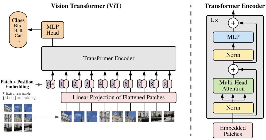
We saw in the first part of this series that residual connections play an important role in ResNets and LSTM cells. This is part of a larger trend where both vision and language models are converging into a single architecture that works well for both. This trend was definitively consolidated by the emergence of vision transformers first proposed by Dosovitskiy et. al. from Google Research team in a paper titled “An Image Is Worth 16×16 Words: transformers For Image Recognition At Scale”[3]. In this paper, the authors applied the encoder block of the transformer architecture to the problem of image classification and found surprising results. We will refer to this as ‘the ViT paper’ in our discussion.

The architecture of the vision transformer model is shown in figure 2.  The caption of the figure contains several terms like class token, and position embedding, which are also present in figure 1. These are the common components of the transformer architecture other than MHSA. Let us introduce them in detail in the context of computer vision.

Patch Embeddings

Transformer models process inputs as words or tokens. If we want to apply transformers to image recognition, the first question to ask is ‘what is the equivalent of words in images?’ There are several choices, such as treating each pixel as a word. However, we note that the computational complexity of calculating the attention matrix is N² where N is the sequence length. If we treat each pixel as a separate word, then assuming a relatively small image size of 100×100, the attention matrix will be of size 10000×10000. This is obviously unmanageable even for the largest GPUs.

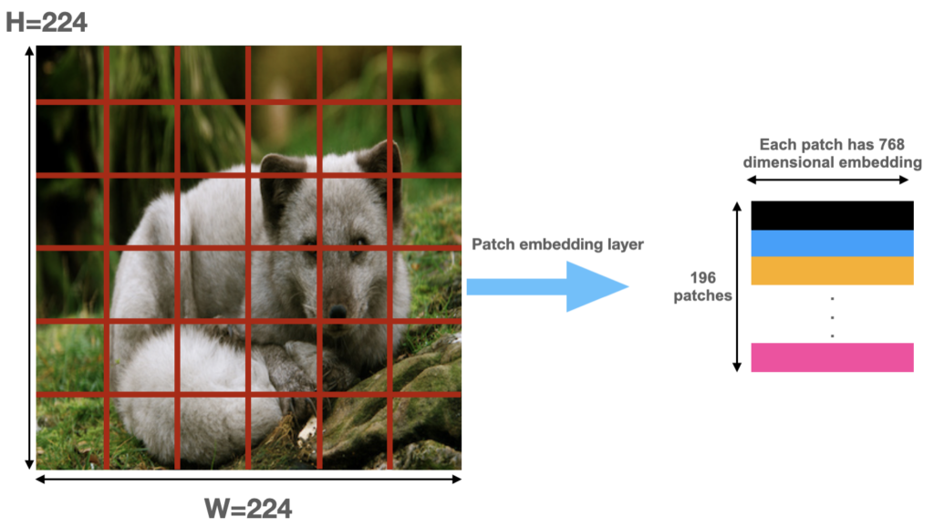
A more moderate choice is to treat a patch of some size, say 16×16, as one word. Thus,  as shown in figure 3, the RGB image of size WxHx3 is divided up into patches, each of size wxhx3. Each patch is flattened and passed through a dense layer without activation, called an embedding layer. The same weights are reused for all patches of the image. The embedding layer transforms the patch into a hidden, learned representation of dimension d_in. Finally, note that before creating the patches, the input image is preprocessed by subtracting the mean and dividing by the standard deviation, just like for any other image classification model.

Let us take the example of the imagenet dataset. As shown in figure 4, an image of size 224×224 pixels (W=H=224) is divided up into patches of size 16×16 (w=h=16). Thus, 14×14 (since 224/16=14) or a total of 196 patches are created from one image. In terms of tensor sizes, assuming a batch size of 1, the input image is of size [1, 3, 224, 224] while after patch embedding, the tensor has size [1, 196, d_in]. For example, d_in = 768 in the base vision transformer model.

Classification Token

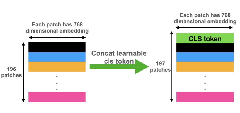
Computer vision has enjoyed the benefits of transfer learning for a long time. However, even as late as 2018, NLP models could not effectively be pre-trained on some datasets and fine-tuned on another for a different task. This changed with the introduction of Bidirectional Encoder Representations from Transformers or BERT. BERT framed the pre-training task as a classification problem. To let the transformer model perform classification, an extra token called the class token was used.

Vision transformers adopt this concept from BERT. The idea is to concatenate a learnable patch to the beginning of the patch sequence, as shown in figure 5. This patch is used read out the classification output at the end of the model, as we will explain in section 2.6. In terms of tensor sizes, continuing with our example of an image, the size before concatenation was [1,196,768]. After concatenating a learnable parameter (nn.Parameter in PyTorch) called class token, the resulting tensor has a size [1,197,768]. This is the size of the input tensor to the transformer model. Thus, recalling the notation from the first part of this series, N=197 and d_in=768.

 Position Embedding

As we learned in the previous part of this series of posts, the vanilla self-attention mechanism does not have any concept of temporal order among its inputs. All patches or words are treated equally. This is a problem since the order of patches and words really matters in both NLP and computer vision. Thus, to allow the transformer to learn to differentiate between patches at different locations, we add something called position embedding to the inputs.

There are many kinds of position embeddings in the NLP literature such as the sine/cosine embeddings and learnable embeddings. Vision transformers work about the same with either of these types. So, we will work with learnable position embeddings.

As shown in figure 6, a position embedding is just a learnable parameter. Continuing with our example of images of size 224×224, recall that after concatenating the classification token, the tensor has size [1, 197, 768]. We instantiate the position embedding parameter to be of the same size and add the patches and position embedding element-wise. The resulting sequence of vectors is then fed into the transformer model.

Layer Normalization

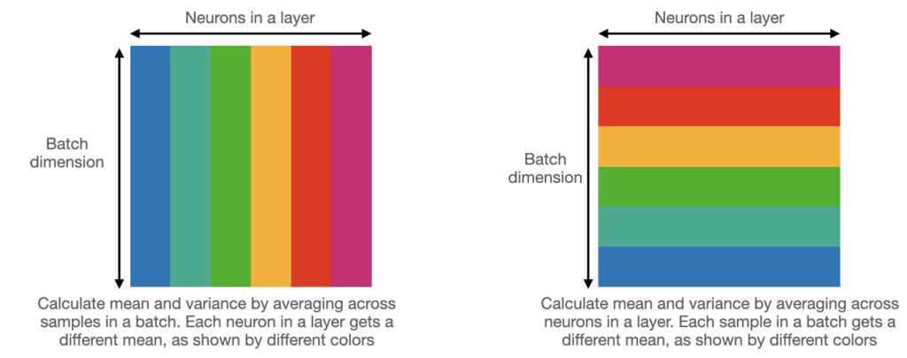
Layer normalization, first proposed by the legendary Professor Geoffrey Hinton’s lab, is a slightly different version of batch normalization. We are all familiar with batch norm in the context of computer vision. However, batch norm cannot be directly applied to recurrent architectures. Moreover, since the mean (μ) and standard deviation (σ) statistics in batch norm are calculated for a mini-batch, the results are dependent on the batch size. As shown in figure 7, layer normalization overcomes this problem by calculating the statistics for the neurons in a layer rather than across the mini batch. Thus, each sample in the mini batch gets a different μ and σ, but the mean and std deviation are the same for all neurons in a layer.

The thing to note is that for typical model sizes, layer norm is slower than batch norm. Thus, some architectures like DEST (which are designed for speed, but we will not introduce them here), use engineering tricks to use batch norm while keeping the training stable. However, for most widely used vision transformers, layer norm is used and is quite critical for their performance.

Multi-Layer Perceptron

As you can see from figure 1 and 2, the encoder layer of the transformer architecture has a feed-forward or MLP module. This is a short sequential module consisting of:

1. A linear layer that projects the output of the MHSA layer into higher dimensions (d_mlp>d_in)
2. An activation layer with GELU activation (GELU(x) = xɸ(x), where ɸ(x) is the cumulative distribution function of the standard gaussian distribution)
3. A dropout layer to prevent overfitting
4. A linear layer to the projects the output back to the same size as the output of the MHSA layer.
5. Another dropout layer to prevent overfitting.

Classification Head

We remarked in the above section on ‘classification token’ that a learnable parameter called a classification token is concatenated to the patch embeddings. This token becomes a part of the vector sequence fed into the transformer model and evolves with self-attention. Finally, we attach a small MLP classification head on top of this module and read the classification results from it. This is just a vanilla dense layer with the number of neurons equal to the number of classes in the dataset. So, for example, continuing with our example of d_in=768, for imagenet dataset, this layer will take in a vector of size 768 and output 1000 class probabilities.

Note that once we have obtained the classification probabilities from the MLP head on top of the classification token, the outputs from all other patches is IGNORED! This seems quite unintuitive and one may wonder why the classification token is required at all. After all, can’t we average the outputs from all the other tokens and train an MLP on top of that, much like what we do with ResNets? Yes, it is quite possible to do so and it works just as well as the classification token approach. Just note that a different, lower learning rate is required to get this to work.

Putting everything together

We now have all the components required to implement a vision transformer. Let us summarize all the components of the ViT architecture:

1. The input images to a ViT model are first pre-processed with mean and standard deviation scaling, just like any other vision model.
2. The images in a batch are then split up into patches
3. The patches are linearly embedded with a learnable layer as explained in section 2.1
4. A learnable parameter called classification token is concatenated to the patch embeddings, as explained in section 2.2.
5. Another learnable parameter called position embedding is added element wise to the patch embeddings (with cls token).
6. The resulting sequence of vectors is fed into a transformer encoder layer. There are L such layers (typically L=12 or 24). The output of each encoder layer has the same shape as the input.
7. Every layer of the encoder consists of:
   • A layer normalization module
   • Multi headed self attention (MHSA) module, explained in previous post
   • Residual connection from the input of the layer to the output of the MHSA module
   • Another layer normalization, and finally
   • The Multi-layer perceptron module explained in the subsection 2.5

1. Finally, a classification head is attached to the top of the output corresponding to the class token which outputs the probabilities for each class.

Implementing The Vision Transformer in PyTorch

Implementing MHSA module

Since we had already introduced the multi-headed self-attention module in great detail in the first part of this series, we have not mentioned it at all in this post. However, to reiterate, the attention mechanism lies at the core of transformer models. Therefore, to begin, we will show the implementation of the MHSA module.

Click here to download the source code to this post

from torch import nn
from einops.layers.torch import Rearrange

class MultiHeadedSelfAttention(nn.Module):
 def __init__(self, indim, adim, nheads, drop):
  '''
  indim: (int) dimension of input vector
  adim: (int) dimensionality of each attention head
  nheads: (int) number of heads in MHA layer
  drop: (float 0~1) probability of dropping a node
  
  Implements QKV MSA layer
  output = softmax(Q*K/sqrt(d))*V
  scale= 1/sqrt(d), here, d = adim
  '''
  super(MultiHeadedSelfAttention, self).__init__()
  hdim=adim*nheads
  self.scale= hdim** -0.5 #scale in softmax(Q*K*scale)*V
  self.key_lyr = self.get_qkv_layer(indim, hdim, nheads)
  #nn.Linear(indim, hdim, bias=False) 
  #there should be nheads layers
  self.query_lyr=self.get_qkv_layer(indim, hdim, nheads)
  self.value_lyr=self.get_qkv_layer(indim, hdim, nheads)
  
  self.attention_scores=nn.Softmax(dim=-1)
  self.dropout=nn.Dropout(drop)
  
  self.out_layer=nn.Sequential(Rearrange('bsize nheads indim hdim -> bsize indim (nheads hdim)'),
  nn.Linear(hdim, indim),
  nn.Dropout(drop))
 
 def get_qkv_layer(self, indim, hdim, nheads):
  '''
  returns query, key, value layer (call this function thrice to get all of q, k & v layers)
  '''
  layer=nn.Sequential(nn.Linear(indim, hdim, bias=False),
  Rearrange('bsize indim (nheads hdim) -> bsize nheads indim hdim', nheads=nheads))
  
  return layer

 def forward(self, x):
  query=self.key_lyr(x)
  key=self.query_lyr(x)
  value=self.value_lyr(x)
  
  dotp=torch.matmul(query, key.transpose(-1, -2))*self.scale
  
  scores=self.attention_scores(dotp)
  
  scores=self.dropout(scores)
  
  weighted=torch.matmul(scores, value)
  
  out=self.out_layer(weighted)
  
  return out

This is just a copy of what we implemented in the earlier post, so if you are rusty on the details, please refer to that post.

Implementing transformer encoder

With the MHSA layer handy, implementing the rest of the encoder layers is quite straightforward. We use the sequence of layers mentioned in bullet point #7 of section 2.7.

class TransformerEncoder(nn.Module):
 '''
 Although torch has a nn.Transformer class, it includes both encoder and decoder layers 
 (with cross attention). Since ViT requires only the encoder, we can't use nn.Transformer.
 So, we define a new class
 '''
 def __init__(self, nheads, nlayers, embed_dim, head_dim, mlp_hdim, dropout):
  '''
  nheads: (int) number of heads in MSA layer
  nlayers: (int) number of MSA layers in the transformer
  embed_dim: (int) dimension of input tokens
  head_dim: (int) dimensionality of each attention head
  mlp_hdim: (int) number of hidden dimensions in hidden layer
  dropout: (float 0~1) probability of dropping a node
  '''
  super(TransformerEncoder, self).__init__()
  self.nheads=nheads
  self.nlayers=nlayers
  self.embed_dim=embed_dim
  self.head_dim=head_dim
  self.mlp_hdim=mlp_hdim
  self.drop_prob=dropout
  
  self.salayers, self.fflayers=self.getlayers()

 def getlayers(self):
  samodules=nn.ModuleList()
  ffmodules=nn.ModuleList()
  
  for _ in range(self.nlayers):
   sam=nn.Sequential(
    nn.LayerNorm(self.embed_dim),
    MultiHeadedSelfAttention(
     self.embed_dim, 
     self.head_dim, 
     self.nheads, 
     self.drop_prob
     )
    )
   
   samodules.append(sam)

   ffm=nn.Sequential(
    nn.LayerNorm(self.embed_dim),
    nn.Linear(self.embed_dim, self.mlp_hdim),
    nn.GELU(),
    nn.Dropout(self.drop_prob),
    nn.Linear(self.mlp_hdim, self.embed_dim),
    nn.Dropout(self.drop_prob)
    )

   ffmodules.append(ffm)
  
  return samodules, ffmodules

 def forward(self, x):
  for (sal,ffl) in zip(self.salayers, self.fflayers):
   x = x+sal(x)
   x = x+ffl(x)
  
  return x

Implementing Vision Transformer class

The core of the vision transformer has already been built. Now, with patch embedding, class token and position embedding we put the scaffolding around it to define the vision transformer class. The constructor to the class takes the following arguments:

1. Size of input images (typically, 224×224 for imagenet, more about this soon)
2. Patch size (typically 16×16, we assume w=h for simplicity)
3. Embedding dimension (typically, d_in=768)
4. Number of encoder layers in the transformer model (typically, L=12)
5. Number of attention heads in the MHSA layer (typically 12)
6. Probability of dropping a neuron in dropout layers (typically 0.1)
7. The dimensionality of the attention layers (typically, d_attn=64)
8. The dimensionality of the expanded representation in MLP head (d_mlp = 3072)
9. Number of classes in the dataset (typically, 1000 for imagenet)

We have mentioned the typical values for the base vision transformer model in parentheses. These arguments are passed as a dictionary.

Let us look at the constructor.

class VisionTransformer(nn.Module):
 def __init__(self, cfg):
  super(VisionTransformer, self).__init__()

  input_size=cfg['input_size']
  self.patch_size=cfg['patch_size']
  self.embed_dim=cfg['embed_dim']
  salayers=cfg['salayers']
  nheads=cfg['nheads']
  head_dim=cfg['head_dim']
  mlp_hdim=cfg['mlp_hdim']
  drop_prob=cfg['drop_prob']
  nclasses=cfg['nclasses']
  
  self.num_patches=(input_size[0]//self.patch_size)*(input_size[1]//self.patch_size) + 1

  self.patch_embedding=nn.Sequential(
   Rearrange('b c (h px) (w py) -> b (h w) (px py c)', px=self.patch_size, py=self.patch_size),
   nn.Linear(self.patch_size*self.patch_size*3, self.embed_dim)
   )

  self.dropout_layer=nn.Dropout(drop_prob)

  self.cls_token = nn.Parameter(torch.randn(1, 1, self.embed_dim))
  # similar to BERT, the cls token is introduced as a learnable parameter 
  # at the beginning of the ViT model. This token is evolved with self attention
  # and finally used to classify the image at the end. Tokens from all patches 
  # are IGNORED.

  self.positional_embedding=nn.Parameter(torch.randn(1, self.num_patches, self.embed_dim))
  #Learnable position embedding

  self.transformer=TransformerEncoder(
   nheads=nheads, 
   nlayers=salayers, 
   embed_dim=self.embed_dim,
   head_dim=head_dim,
   mlp_hdim=mlp_hdim,
   dropout=drop_prob
   )
  
  self.prediction_head=nn.Sequential(nn.LayerNorm(self.embed_dim), nn.Linear(self.embed_dim, nclasses))

Implementing Forward Method

With all these details under our belt, the forward method of the vision transformer model can be implemented by following the prescription in section 2.7. 

One detail to note is that the learnable position embeddings have a specific size determined by image size and patch size at the time of constructing the model. During inference, we may get an image that is of a different size than training. Transformers have no problem in dealing with images of any size. 

However, since we perform element wise addition of position embeddings (which have a constant size), they cannot deal with inputs of any arbitrary size. To overcome this, we simply linearly interpolate the position embeddings to be of the same size as the input image patches. The authors of ViT paper do not present any concrete results showing whether or not this hurts performance, but an empirical study done by the author of this blog post shows that inferring on images of larger size than training significantly hurts performance. Nevertheless, we follow the prescription provided by Dosovitskiy et. al.

def forward(self, x):
 #x is in NCHW format
 npatches=(x.size(2)//self.patch_size)*(x.size(3)//self.patch_size) + 1
 embed = self.patch_embedding(x)
 
 x=torch.cat((self.cls_token.repeat(x.size(0),1,1), embed), dim=1)
 #repeat class token for every sample in batch and cat along patch dimension, so class token is trated just like any patch
 
 if npatches==self.num_patches:
  x+=self.positional_embedding
  #this will work only if size of input image is same as that specified in the constructor
 else:
  interpolated=nn.functional.interpolate(
   self.positional_embedding[None], #insert dummy dimension
   (npatches, self.embed_dim), 
   mode='bilinear'
   ) 
  #we use bilinear but only linear interp will be used
  x+=interpolated[0] #remove dummy dimension

 x=self.dropout_layer(x)
 
 x= self.transformer(x)
 
 x= x[:,0,:] 
 #use the first token for classification and ignore everything else
 
 pred=self.prediction_head(x)

 return pred

Finally, we can instantiate the vision transformer model and do a dummy test to see that everything works as expected. To make managing the configurations easier, we have implemented the base, large and huge configs in a separate file called vitvonfigs.py

base={
 'input_size':[224,224,3],
 'patch_size':16,
 'embed_dim':768,
 'salayers':12,
 'nheads':12,
 'drop_prob':0.1,
 'head_dim':64,
 'mlp_hdim':3072,
 'nclasses':1000
}

large={
 'input_size':[224,224,3],
 'patch_size':16,
 'embed_dim':1024,
 'salayers':24,
 'nheads':16,
 'drop_prob':0.1,
 'head_dim':64,
 'mlp_hdim':4096,
 'nclasses':1000
}

huge={
 'input_size':[224,224,3],
 'patch_size':14,
 'embed_dim':1280,
 'salayers':32,
 'nheads':16,
 'drop_prob':0.1,
 'head_dim':80,
 'mlp_hdim':5120,
 'nclasses':1000
}

Using these configs, you can verify that the number of parameters of the model is almost exactly as that reported in Table 1 of the ViT paper.

Training the Vision Transformer

Implementing a vision transformer is not enough. We need to train it as well. We will use the imagenet dataset and train the base configuration of the ViT model. Rather than writing the whole data processing pipeline and a bunch of boiler plate to run through epochs and batches, we will use a simple library developed by the author of this blog post, called DarkLight. We note that this is just one of the ways of training the model. Please feel free to experiment and integrate the vision transformer model into a training pipeline of your choice.

I created the dark light library[4] primarily for fast knowledge distillation in PyTorch, but it can just as easily be used for training standalone models. Note that the rest of the code in this section requires a CUDA enabled GPU, as it is not practical to train large models purely on a CPU. You will also need TensorRT to be installed for dark light to work.

Install dark light with 

pip install darklight

The library implements a data loader for ImageNet, handles all the training loop, can perform mixed precision training and can even use TensorRT for training (but that is perhaps a discussion for another blog post). The training script is thus very simple:

import darklight as dl
import torch
from vit import VisionTransformer
import vitconfigs as vcfg

net=VisionTransformer(vcfg.base)
dm=dl.ImageNetManager('/sfnvme/imagenet/', size=[224,224], bsize=128)

opt_params={
 'optimizer': torch.optim.AdamW,
 'okwargs': {'lr': 1e-4, 'weight_decay':0.05},
 'scheduler':torch.optim.lr_scheduler.CosineAnnealingWarmRestarts,
 'skwargs': {'T_0':10,'T_mult':2},
 'amplevel': None
 }
trainer=dl.StudentTrainer(net, dm, None, opt_params=opt_params)
trainer.train(epochs=300, save='vitbase_{}.pth')

Since we (and perhaps you) do not have the training resources of Google, we will review the results presented by the authors and not trained by us. At the end of this post, we will introduce some great resources to find pre-trained ViT models.

Results from The Vision Transformer Paper

At the start of this series, we stated that transformers have taken over computer vision and are behind some of the most impressive recent advances in both computer vision and NLP. Now, that we have a firm understanding of the transformer architecture, let us compare the performance of these models, as reported by Dosovitskiy et. al.

To start with, let us note that there are 3 variants of the ViT model that the authors report about, the base, large and huge models, as shown in figure 8.

The results on a large number of datasets show that vision transformers, especially the large and huge models outperform other state of the art methods. The authors pre-train all models on Google’s internal JFT-300 dataset which contains 300 million images, and then fine-tune on smaller public datasets. As shown in figure 9 (table 2 from the paper), the ViT models outperform even the largest ResNets by a healthy margin. However, this is not the full story. Like Vaswani et. al. reported for NLP tasks, vision transformer models require substantially fewer resources to train for computer vision tasks.

In particular, we see that the large model with a patch size of 16 achieves better performance on ImageNet than the Big Transfer (BiT), a large ResNet model (87.76% v/s 87.54%), while using about 14x less (9.9k v/s 0.68k TPU days) training resources!! The huge model also requires about 4x fewer training resources than BiT but outperforms it by 1%, which is a big improvement on the ImageNet dataset.

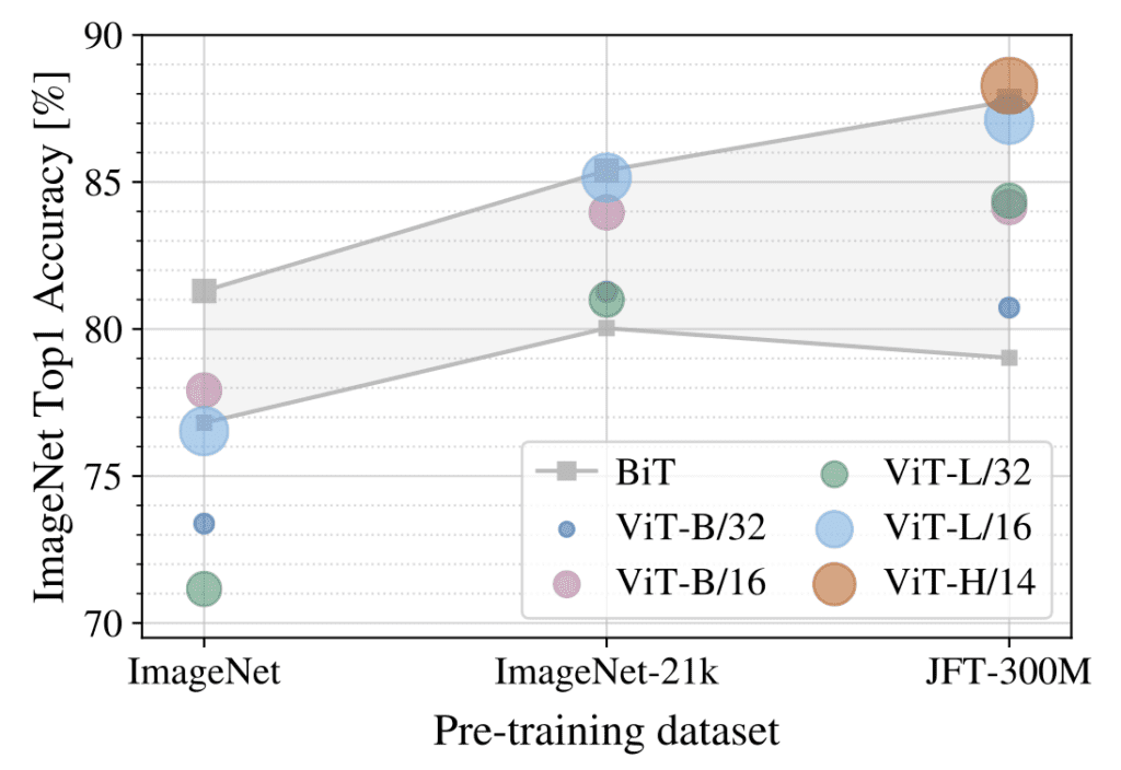
Here is another important result, shown in figure 10. The authors train all models on datasets of varying sizes and evaluate them on ImageNet. Note that the ImageNet dataset has 1.3 million images, while the ImageNet-21k dataset has 15 million images and JFT has 300 million images. The shaded gray area represents the performance band of various configurations of ResNets. The authors found that on smaller datasets, vision transformers perform worse than ResNets. This is expected as convolutional networks have an inductive bias built in, which allows them to learn quickly from small data. 

However, as the size of the datasets increases, these fixed inductive biases hamstring convolutional networks, and transformers with their more general computational architecture and no inductive bias overtake the performance of even the largest ResNets, as shown on the right side of the figure. Moreover, they do so while requiring substantially fewer computational resources to train than comparable ResNets.

This is quite a remarkable result. Recall that transformer models and the attention mechanism were first proposed for NLP tasks and their design is quite different from the conceptually pleasing design of convolutional networks. Even though transformers don’t have the inductive biases of convolutional networks, they manage to beat them in performance given enough data, and they manage to do so while requiring fewer resources to train!! We have only covered the basic image classification model in this blog post, but these performance advantages carry over to other tasks as well. We will explore these tasks and architectures in future posts of this series.

Pre-trained Vision Transformers

There is a famous no-free-lunch theorem in machine learning which implies that there is no single best model for all possible tasks and dataset sizes. Thus, we cannot tell a priori if vision transformers will suit what you are doing. If you want to explore vision transformers and evaluate them on your datasets and projects, here are a few good resources:

1. A GitHub user named lucidrains has an amazing repository called vit-pytorch that implements vision transformers and several variants proposed in the literature. While these are great resources for learning the details of vision transformers, these models are not pre-trained. Link: https://github.com/lucidrains/vit-pytorch

2. An open-source library called torch image models (timm) has pre-trained models for almost all possible variants of vision transformers and all public datasets, including the massive ImageNet-21k dataset with 15 million images. JFT-300M is obviously not included as it is a confidential dataset for Google’s internal team. Ross Wightman, the developer of this library is also quite active in maintaining the library and is worth a follow on Twitter as well. Link to library: https://github.com/rwightman/pytorch-image-models

3. Torchvision is, of course, the most popular PyTorch library for pre-trained computer vision models, and the newer versions of torch vision also contain pre-trained weights for vision transformers.

Summary

In this blog post, we have introduced several new concepts which are unfamiliar to a typical computer vision workflow. To recap, 

1. We built upon the base of multi headed self attention mechanism that we built in the first part of this series. 
2. We quickly reviewed the evolution of ideas in NLP and how Vaswani et. al. proposed a full attention based architecture in their famous ‘Attention is all you need’ paper. 
3. Dosovitskiy et. al. took inspiration from that paper and constructed large vision transformer models using the encoder part of the transformer. 
4. We reviewed the various components of vision transformers, such as patch embedding, classification token, position embedding, multi layer perceptron head of the encoder layer, and the classification head of the transformer model.
5. With everything by our side, we implemented vision transformer in PyTorch. We also briefly saw one way of training the model using dark light library.
6. We then reviewed the results reported in the paper and put them in perspective, and finally ended by reviewing some open-source projects which provide pre-trained models and learning resources.

Congratulations on not giving up and sticking until the end. We hope that vision transformers will be a useful tool in your arsenal of machine learning models. We highly recommend perusing the various papers mentioned in this post. There is a lot to the story of vision transformers, including mobile vision transformers, object detection and image segmentation with transformers and so on, which we will cover in future posts of this series. We hope to see you there.

References

[1] Bahdanu et. al., “Neural Machine Translation by Jointly Learning to Align and Translate”, https://arxiv.org/abs/1409.0473

[2] Vaswani et. al., “Attention Is All You Need”, https://arxiv.org/abs/1706.03762

[3] Dosovitskiy et. al., “An Image Is Worth 16×16 Words: transformers For Image Recognition At Scale”, https://arxiv.org/abs/2010.11929
[4] DarkLight GitHub Repository, https://github.com/dataplayer12/darklight