In an earlier post, we covered the problem of Multi Label Image Classification (MLIC) for Image Tagging.
Recall that MLIC is an image classification task but unlike multi-class image classification or multi-output image classification, the number of labels an image can have isn’t fixed.
The differences are show in the table below.
| Type | Total Number of classes | Number of outputs |
| Binary Classification | 2 | 1 |
| Multi-class classification | N | 1 |
| Multi-output classification | N | Fixed |
| Multi-label classification | N | Variable |
A classical approach to solving this task would be to use a standard classification network with a Binary Cross-Entropy (BCE) or SoftMargin loss as we did in the earlier post.
Let’s dive a little deeper into the task and consider more sophisticated (and effective) approaches to solving this problem.
Labels are Correlated
Let’s begin by observing Figure 1 below. It shows an image and tags corresponding to the image on top of the image.
Notice some of the tags are not independent. For example, if there is a sky label for an image, the probability of seeing the cloud or sunset labels for the same picture are high. The same holds true for the labels ocean, lake, and water labels.
It’s logical to assume that labels aren’t independent since in real life such objects or aspects are interconnected.
This intuition is a core idea behind the most recent papers for MLIC. Researchers are trying to use prior knowledge about connections between labels to get better results.
In the paper “Multi-Label Image Recognition with Graph Convolutional Networks” the authors use Graph Convolution Network (GCN) to encode and process relations between labels, and as a result, they get a 1–5% accuracy boost.
The paper “Cross-Modality Attention with Semantic Graph Embedding for Multi-Label Classification” proposes the further development of this idea. The authors added special attention to the approach from the former paper and obtained an additional 1–5% accuracy boost.
Graph
Before we move to the explanation of what GCNs are and how they’re applied to the task at hand, we should understand what are graphs and how are they related to our problem.
A graph is a structure that encodes relationships between objects.
In a graph, objects are represented using “nodes” while an “edge” between the nodes represents the relationship between the pair of the nodes.
The edges may have their own weights to represent the strength of relationship between nodes. In such cases, the graph is a weighted graph.
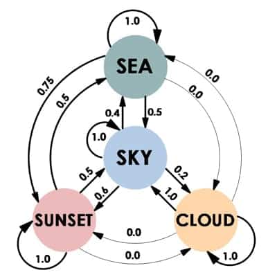
There are many structures that fit this definition, both abstract and practical. Social networks are an obvious example from real-life. A less obvious example may be the routes through a city. Now, let’s look at some synthetical example that illustrates our image tagging task. Imagine we have a dataset with some vacation photos and 4 possible labels: ‘Sea’, ‘Sky’, ‘Sunset’, ‘Cloud’.
We also have 8 data samples with the following labels assigned to them:
1: ‘Sea’, ‘Sky’, ‘Sunset
2: ‘Sky’, ‘Sunset’
3: ‘Sky’, ‘Cloud’
4: ‘Sea’, ‘Sunset’
5: ‘Sunset’, ‘Sea’
6: ‘Sea’, ‘Sky’
7: ‘Sky’, ‘Sunset’
8: ‘Sunset’
We can represent the labels as the graph nodes, but what are the connections between them? We propose to add connections between each pair of labels with weights reflecting the probability of some label’s appearance given that another label is already here.
Let’s elaborate a bit on that. The probability of each label in our dataset would be just the ratio of samples with this label divided by the total number of data samples. We’ve already noticed that some labels often come in pairs. This particular feature can be represented using the conditional probability, that’s P(Lj | Li), which denotes the probability of occurrence of label Lj when label Li appears.
Adjacency matrix
Now let’s take a moment to talk about how we can represent the graph structure to make use of it in our DL pipeline.
There are dozens of ways to represent graphs, but here we want to focus on a popular method that also fits our requirements – adjacency matrix.
For model training, we can compute this matrix based on the training dataset. First, we count the occurrences of label pairs in the training set and get the matrix A∈ R C×C. Here, C is the number of labels, Li is a specific label, and Aij denotes the number of samples with both labels Li and Lj.
| Sea | Sky | Sunset | Cloud | |
|---|---|---|---|---|
| Sea | 0 | 2 | 3 | 0 |
| Sky | 2 | 0 | 3 | 1 |
| Sunset | 3 | 3 | 0 | 0 |
| Cloud | 0 | 1 | 0 | 0 |
We can calculate the number of occurrences for each label Li in the training dataset:
| Sea | Sky | Sunset | Cloud | |
|---|---|---|---|---|
| N | 4 | 5 | 6 | 1 |
Then, by dividing this label co-occurrence matrix row by row (that’s Pi = Ai/Ni), we can get the conditional probabilities for each pair of labels.
| Sea | Sky | Sunset | Cloud | |
|---|---|---|---|---|
| Sea | 0 | 0.4 | 0.5 | 0 |
| Sky | 0.5 | 0 | 0.5 | 1 |
| Sunset | 0.75 | 0.6 | 0 | 0 |
| Cloud | 0 | 0.2 | 0 | 0 |
Pij = P(Lj | Li) means the probability of label Lj when label Li appears.
Lastly, we add self-loops, because the probability of some label being on an image if it’s already here is 1:
P = P + Identity(length(P))
| Sea | Sky | Sunset | Cloud | |
|---|---|---|---|---|
| Sea | 1 | 0.4 | 0.5 | 0 |
| Sky | 0.5 | 1 | 0.5 | 1 |
| Sunset | 0.75 | 0.6 | 1 | 0 |
| Cloud | 0 | 0.2 | 0 | 1 |
And now we have our weighted adjacency matrix which represents a directed weighted graph with 4 nodes and edges weighted according to the probability of each label pair co-occurrence.
Note that probabilities P(Li | Lj) and P(Lj | Li) are not equal and that’s normal.
If there is a Cloud, the probability of having Sky is 1.0. But if there is a sky, the probability of Cloud is 0.2 – the sky may have no clouds.
Graph Convolution vs Convolution
We all know about a standard Convolution layer. It works as a filter and extracts features from numerical data (such as images, signals, etc.). The graph convolution layer has the same logic. It works as a filter and extracts the features from graphs. To draw more parallels between them, it’s better to think about the picture as a graph with adjacent pixels connected by edges.
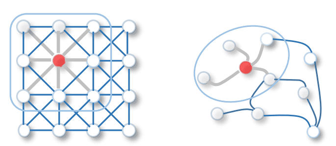
Image credits A Comprehensive Survey on Graph Neural Networks
In the Convolution layer, we use the size of the convolution kernel to indicate the size of the neighborhood (how many pixels will contribute to the resulting value). Similarly, the Graph Convolution layer uses neighbors of a particular graph node to define a convolutional operation in it. Two nodes are neighbors if they have a common edge. In Graph Convolutions a learnable weight is multiplied by features of all the neighbors of a particular node (including the node itself) and some activation function is applied on top of the result. Formally, the result of Graph Convolution applied at node vi with a corresponding feature vector hvi would be:
Here N is an index set of neighborhood nodes of the node vi (it also includes i), W is a learnable weight that is the same for all nodes in the neighborhood, and f is some non-linear activation function.
Let’s now explain what cij is and how to implement this operation.
It’s a constant parameter for the edge (vi, vj) from the symmetrical normalization matrix. We compute this matrix by multiplying inversed degree matrix D and binary adjacency matrix A (we will describe how to get binary adjacency matrix from the weighted one further), so symmetric normalization matrix is computed once for the input graph as follows:
Graph Convolutional Networks
Naturally, we can stack multiple Graph Convolution layers alternating them with activation functions, just like we do in CNNs. Thus we get Graph Convolution Network (GCN).
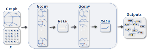
Image credits A Comprehensive Survey on Graph Neural Networks
Let’s now outline the whole GCN pipeline we are going to use in our example. We have a graph with С nodes, and we would like to apply the GCN. The goal of Graph Convolutional operation is to learn a function of input/output features. As input, it takes a С×D feature matrix (D is the dimension of the input features) and a weighted adjacency matrix P that represents the graph structure in a matrix form.
Then several Graph Convolutions are applied sequentially with ReLU as an activation function. The output of Graph Convolutional operation is a СxF feature matrix, where F is the number of output features per node.
class GraphConvolution(nn.Module):
    """
        Simple GCN layer, similar to
        https://arxiv.org/abs/1609.02907
    """
    def __init__(self, in_features, out_features, bias=False):
        super(GraphConvolution, self).__init__()
        self.in_features = in_features
        self.out_features = out_features
        self.weight = Parameter(
                  torch.Tensor(in_features, out_features),
                  requires_grad=True)
        if bias:
            self.bias = Parameter(
                         torch.Tensor(1, 1, out_features),
                         requires_grad=True)
        else:
            self.register_parameter('bias', None)
        self.reset_parameters()

    def reset_parameters(self):
        stdv = 1. / math.sqrt(self.weight.size(1))
        self.weight.data.uniform_(-stdv, stdv)
        if self.bias is not None:
            self.bias.data.uniform_(-stdv, stdv)

    def forward(self, input, adj):
        support = torch.matmul(input.float(),
                               self.weight.float())
        output = torch.matmul(adj, support)
        if self.bias is not None:
            return output + self.bias
        else:
            return output

    def __repr__(self):
        return self.__class__.__name__ + ' (' \
               + str(self.in_features) + ' -> ' \
               + str(self.out_features) + ')'
Label vectorization (GloVe)
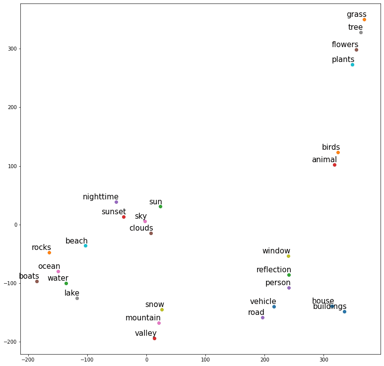
We just discussed how GCNs work and how they take a feature matrix as input with a feature vector per node. In our task though, we don’t have any features for labels, just their names. When working with text in neural networks, a vector representation of words is usually used. Each vector represents a specific word in the space of all words of the corpus (dictionary) on which this space was calculated. The space of words is necessary to find the relationships between the words: the closer the vectors are to each other in this space, the closer their meanings are. Take a look at t-SNE for feature visualization post for ideas on how to build such an image for labels from our small subset of the dataset.
You can see that the words with close meanings (like sky, sun, clouds) are close in the feature space.
There are various approaches to obtaining this space, in our example, we use the GloVe model built on Wikipedia with a feature vector of length 300.
ML-GCN
We are going to implement the approach from the Multi-Label Image Recognition with Graph Convolutional Networks paper. It consists of applying all the steps described earlier:
- Calculate a weighted adjacency matrix from the training set.
- Calculate the matrix with per-label features: X=LxD
- Use vectorized labels X and weighted adjacency matrix P as the input of the graph neural network, and preprocessed image as the input for the CNN network.
- Train the model!
We’d like to discuss several practical tricks left before moving to the implementation of this approach.
When training on real data, usually the following problems arise: overfitting and over-smoothing. The ways to solve them when working with the Multi-Label Graph Convolutional Networks (ML-GCN) are described below.
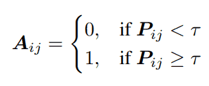
Weighted adjacency matrix thresholding
To avoid overfitting, we filter the pairs in the weighted adjacency matrix that have probabilities lower than a certain threshold τ (we use τ=0.1). Such edges we interpret as being poorly represented or error connections. That may happen, for example, due to the noise in training data. For example, in our case such connections are ‘birds’ and ‘nighttime’: they represent random coincidences rather than real relations.
Over-smoothing problem
After applying a Graph Convolution layer, the feature of the node will be the weighted sum of its own feature and the adjacent nodes’ features.
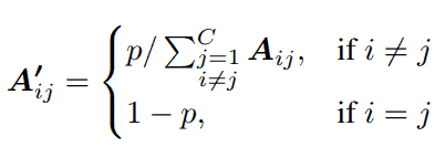
It may result in an over-smoothing of the features in a particular node, especially after applying several layers. To prevent this, we introduce a parameter p that calibrates the weights assigned to the node itself and other correlated nodes. By doing this, when updating the node feature, we will have a fixed weight for the node itself, and the weights for its neighbor nodes will be determined by the neighborhood distribution. When p → 1, the feature of the node itself will not be considered. On the other hand, when p → 0, neighboring information tends to be ignored. In our experiments, we use p=0.25.
Finally, let’s construct the model with GCN. We took the first 4 layers from ResNeXt50 as a visual feature extractor and used multi-layer GCN as a label relationship extractor. Features from the image itself and the labels are then combined via a dot product operation. See the scheme below:
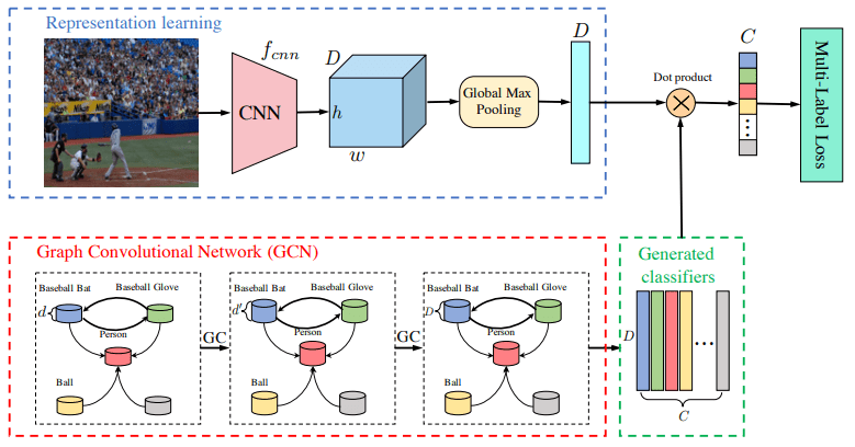
Image credits Multi Label Image Recognition with Graph Convolutional Networks
# Create adjacency matrix from statistics.
def gen_A(num_classes, t, p, adj_data):
    adj = np.array(adj_data['adj']).astype(np.float32)
    nums = np.array(adj_data['nums']).astype(np.float32)
    nums = nums[:, np.newaxis]
    adj = adj / nums
    adj[adj < t] = 0
    adj[adj >= t] = 1
    adj = adj * p / (adj.sum(0, keepdims=True) + 1e-6)
    adj = adj + np.identity(num_classes, np.int)
    return adj

# Apply adjacency matrix re-normalization trick.
def gen_adj(A):
    D = torch.pow(A.sum(1).float(), -0.5)
    D = torch.diag(D).type_as(A)
    adj = torch.matmul(torch.matmul(A, D).t(), D)
    return adj


class GCNResnext50(nn.Module):
    def __init__(self, n_classes, adj_path, in_channel=300,
                 t=0.1, p=0.25):
        super().__init__()
        self.sigm = nn.Sigmoid()

        self.features = models.resnext50_32x4d(pretrained=True)
        self.features.fc = nn.Identity()
        self.num_classes = n_classes

        self.gc1 = GraphConvolution(in_channel, 1024)
        self.gc2 = GraphConvolution(1024, 2048)
        self.relu = nn.LeakyReLU(0.2)
        # Load statistics data for adjacency matrix
        with open(adj_path) as fp:
            adj_data = json.load(fp)
        # Compute adjacency matrix
        adj = gen_A(n_classes, t, p, adj_data)
        self.A = Parameter(torch.from_numpy(adj).float(),
                           requires_grad=False)

    def forward(self, imgs, inp):
        # Get visual features from image
        feature = self.features(imgs)
        feature = feature.view(feature.size(0), -1)

        # Get graph features from graph
        inp = inp[0].squeeze()
        adj = gen_adj(self.A).detach()
        x = self.gc1(inp, adj)
        x = self.relu(x)
        x = self.gc2(x, adj)

        # We multiply the features from GCN and CNN in order to
        # take into account the contribution to the prediction of
        # classes from both the image and the graph.
        x = x.transpose(0, 1)
        x = torch.matmul(feature, x)
        return self.sigm(x)
Accuracy comparison with the earlier post
Comparing ML-GCN with the naive approach from the earlier post, we find that ML-GCN approach is more accurate:
| ResNeXt50 | ML-GCN | Difference | |
|---|---|---|---|
| macro f1-score | 0.54 | 0.59 | +0.05 |
| microf1-score | 0.7 | 0.72 | +0.02 |
| sample f1-score | 0.67 | 0.7 | +0.03 |
Summary
In this post, we’ve shown how to represent the graph structure in CNN, and how Graph Convolutional Networks works. We also applied them to a real-life task: multi-label classification of images. GCN has significantly increased the baseline accuracy there proving that GCNs are a powerful tool that can be used to further improve the quality and performance of a broad range of deep learning tasks.
For further information please check the links below.
Additional links
Semi-supervised classification with graph convolutional networks
A Comprehensive Survey on Graph Neural Networks
Multi-Label Image Recognition with Graph Convolutional Networks
Cross-Modality Attention with Semantic Graph Embedding for Multi-Label Classification
Simplifying Graph Convolutional Networks













100K+ Learners
Join Free OpenCV Bootcamp3 Hours of Learning