Depth estimation is a critical task for autonomous driving. It’s necessary to estimate the distance to cars, pedestrians, bicycles, animals, and obstacles.
The popular way to estimate depth is LiDAR. However, the hardware price is high, LiDAR is sensitive to rain and snow, so there is a cheaper alternative: depth estimation with a stereo camera. This method is also called stereo matching.

In general, the idea behind the stereo matching is pretty straightforward.
We have two cameras with collinear optical axes, which have a horizontal displacement only. We can find a corresponding pixel on the right camera frame for every pixel on the left camera frame. We can estimate the point’s depth if we know the distance between pixels related to this point on the left and right frames. As one can see from the depth of the point is inversely proportional to the distance between the images of this point. This distance is called a disparity:

Classical Approaches For Stereo Matching

A classical approach to disparity estimation consists of the following steps:

Extract features from the image to get more valuable information than raw color intensities and improve the point’s matching.
Construct the cost volume to estimate how the left and the right feature maps match each other on different disparity levels. For example, we can use absolute intensity differences or cross-correlation.
Calculate the disparity from the cost volume using the disparity computation module. For example, a brute-force algorithm can look for a disparity level at which left and right feature maps match best.
Refine the disparity if the initially predicted disparity map is too coarse.

You can refer to the survey by Scharstein and Szeliski that provides an overview of the pre-deep-learning methods for stereo matching.

Datasets for stereo matching

Data plays a crucial role in computer vision, so a few words about the datasets for stereo matching:

Middlebury dataset is one of the first datasets for this task. It contains 33 static indoor scenes. The paper describes the dataset acquisition.
The large synthetic SceneFlow dataset contains more than 39 thousand stereo frames in 960×540 resolution. Many authors used it for the pretraining of stereo-matching neural networks. There is a detailed description of the dataset in the paper.
KITTI is a popular benchmark for an autonomous driving scenario. Data is collected from a moving vehicle, and a LiDAR estimates depth.

Deep Learning-Based Approaches for Stereo Matching

Nowadays, deep learning methods combine many of the steps described above into an end-to-end algorithm. A very early example is GCNet. StereoNet and PSMNet follow the same idea. We can focus deeply on the PSMNet approach.

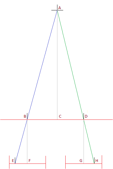
You can see the list of its building blocks in Figure 1.

<strong>Figure 2<strong> Architecture of PSMNet

The approach uses backbones with shared weights to extract features from both left and right images. Interestingly, the authors adopt the Spatial Pyramid Pooling block from semantic segmentation nets to combine features from different scales.

Next, the authors concatenate features from the left image with features from the right image shifted horizontally by $disp$ pixels. They use $disp$ in the range $[0, max disparity]$ and combine the result into a 4D volume.

As the next step, 3D convolution encoder-decoder architecture improves and reduces cost volume. The final layer is a 3D convolution that produces a feature map with $H \times W \times (max disparity + 1)$ size.

Finally, the authors apply the soft argmin function to predict the disparity. Every channel of the output $H \times W \times (max disparity + 1)$ feature map represents a different disparity. The authors normalize the probability volume across the disparity dimension with the softmax operation, $\sigma(\cdot)$ . They combine the disparities, $d$ , with the weights corresponding to their probabilities. The formula below represents this operation:

$soft argmin = \sum_{d=0}^{D_max} d \times \sigma(-c_d)$

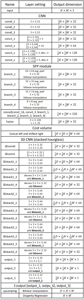
If we look at the KITTI benchmark results in Figure 3 (dated by the middle of August 2020), we can notice that the top stereo-matching approaches are slow. The fastest work from the top-10 on the KITTI 2015 benchmark provides only 3.3 frames per second using GPU. The reason is the top models use 3D convolutions to improve the quality, but the cost is the algorithm’s speed.

top kitti leaderboard — <strong>Figure 3<strong> Top 10 results on the KITTI 2015 benchmark

There are stereo-matching methods that use a correlation layer (MADNet, DispNetC), but they lose the battle for the quality to 3D convolution-based methods.

One of the recent approaches trying to achieve state-of-the-art results while being significantly faster than other methods is AANet.

AANet

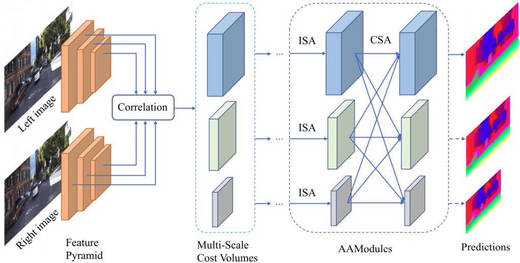
The general method’s architecture is the following:

A shared network (feature extractor) extracts feature pyramids from the left and right images: ${\{ F_l^{s}\}_{s=1}^S}$ and ${\{ F_r^{s}\}_{s=1}^S}$ , correspondingly.
$S$ denotes the number of scales, $s$ is the scale index, and $s=1$ represents the largest scale.
A correlation layer constructs multi-scale 3D cost volumes:
$C^s(d, h, w) = \frac{1}{N} \big \langle F_l^{s}(h, w), F_r^{s}(h, w - d) \big \rangle,$
where $\big \langle \cdot, \cdot \big \rangle$ is an inner product of two feature vectors, $N$ is a number of channels of extracted features, $C^s(d, h, w)$ is the matching cost at the location $(h, w)$ for disparity candidate $d$ . This correlation layer is similar to the one from DispNetC.
Several Adaptive Aggregation Modules aggregate cost volumes. These modules replace 3D encoder-decoder network used earlier in [GCNet, StereoNet, PSMNet],
At the final step, the refinement module upsamples low-resolution disparity prediction to the original resolution. AANet uses two refinement modules proposed in StereoDRNet.

The figure below depicts AANet architecture.

Adaptive Aggregation Module (AAModule)

Let’s focus on the Adaptive Aggregation Module (AAModule) that is the major novelty of the paper.

It consists of two major parts:

Intra-Scale Aggregation (ISA)
Cross-Scale Aggregation (CSA)

Intra-Scale Aggregation

Deep learning-based stereo matching methods usually perform window-based cost aggregation:

$\tilde{C(}d,p) = \sum_{q \in N(p)} w(p, q) C(d, q),$

where $\tilde{C(}d,p)$ is an aggregated cost at pixel $p$ for disparity candidate $d$ , pixel $q$ belongs to the neighbors $N(p)$ of $p$ , $w(p, q)$ is the aggregation weight, and $C(d, q)$ is the raw matching cost at pixel $q$ for disparity candidate $d$ .

However, it should work well only when the disparity is continuous, but the object boundaries violate this assumption.

That’s why we should design the weighting function carefully and eliminate the influence of pixels on the disparity discontinuities.
This problem is called an edge-fattening issue.

The authors of AANet propose the adaptive sampling method instead of regular sampling used in simple 2D and 3D convolutions to cope with the edge-fattening problem. The idea is identical to deformable convolutions.

The cost aggregation strategy for AANet learns an additional offset to the regular sampling location:

$\tilde{C(}d,p) = \sum_{k=1}^{K^2} w_k \cdot C(d, p + p_k +\Delta{p_k}),$

where $K^2$ is the number of sampling points, $w_k$ is the aggregation weight for $k$ -th point, $p_k$ is the fixed offset to $p$ , $\Delta{p_k}$ is the learnable offset.

The authors also make convolution weights content-adaptive with the modulation mechanism from Deformable ConvNets v2: More Deformable, Better Results.

The final cost aggregation formulation looks as follows:

$\tilde{C(}d,p) = \sum_{k=1}^{K^2} w_k \cdot C(d, p + p_k +\Delta{p_k}) \cdot m_k,$

where $m_k$ is a content-specific weight at pixel $k$ .

The only difference with deformable convolution is the number of groups. Feature map consists of G groups, and each group of channels has its own offsets $\Delta{p_k}$ and weights $m_k$ , unlike the original implementation of deformable convolution, where all channels in the feature map share the same offsets and weights.

Cross-Scale Aggregation

The authors of AANet propose to combine cost aggregation on multiple scales. Cost aggregation on the high resolution is required to cope with fine details, while cost aggregation on the coarse resolution is beneficial for low-texture and textureless regions.

AANet combines the features in the following way:

$\hat{C^s} = \sum_{k=1}^{S} f_k({\tilde C}^k), s = 1, 2, ..., S,$

where $\hat{C}$ is the resulting cost volume after cross-scale cost aggregation, $\tilde{C^k}$ is the aggregated cost volume at scale $k$ , $f_k$ is a function to combine cost volumes with different shapes.

The idea here is identical to the concept of HRNet and $f_k$ is adopted from that paper.

$f_k = \begin{cases} I, \; k=s, \\ (s - k) \; stride - 2 \; 3\times 3 \; convs, \; k<s, \\ upsampling \bigoplus 1 \times 1 \; conv, \; k>s, \end{cases}$

where $I$ is an identity function, $(s-k) 3\times3$ convolutions with $stride=2$ are used to downsample a feature map $2^{s-k}$ times, $\bigoplus$ is a bilinear upsampling.

The only difference with HRNet is the number of channels for feature maps with smaller resolutions. HRNet has more channels in low-resolution feature maps than high-resolution ones as feature extractors typically provide them this way. In contrast, AANet has fewer channels in coarse-scale feature maps than in high-scale ones. The reason is that the number of channels represents the number of disparity candidates, so coarse representation needs fewer disparity levels.

Results

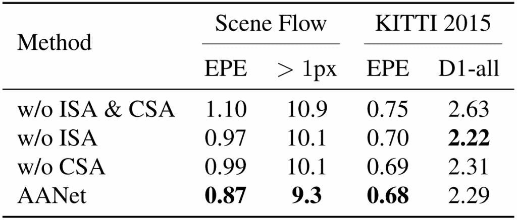
The authors make an ablation study to prove the importance of the proposed modules. They remove ISA and CSA modules from AANet, and the quality worsens.

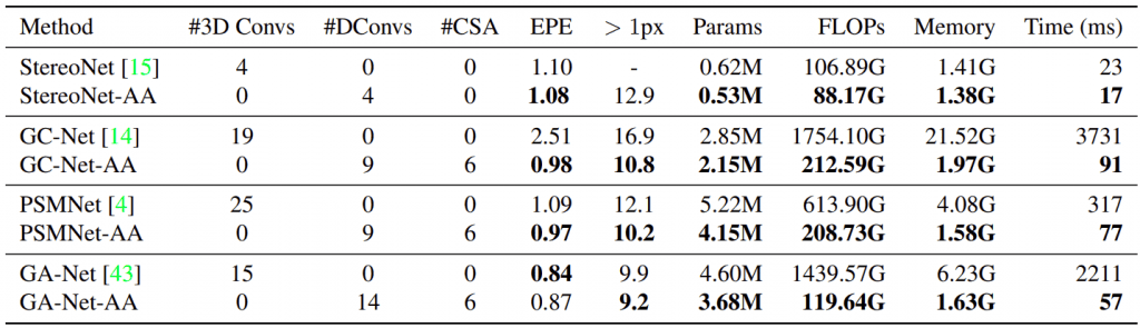
isa and csa ablation study depth estimation opencv — <strong>Figure 5<strong> Ablation study of ISA and CSA modules

They also replaced 3D convolution encoder-decoders with ISA & CSA modules into several popular approaches and achieved a significant speedup and lower memory consumption.
More than that, quality becomes better for StereoNet, GCNet, and PSMNet. There is only a negligible quality drop for GANet.
The authors denote modified architectures with AA suffix.

popular approaches with isa and csa depth estimation from single image python — <strong>Figure 6<strong> Integration of ISA and CSA modules into deep learning based stereo matching methods Inference time is measured with <em>576×960<em> resolution on NVIDIA V100 GPU

The authors modified GANet-AA’s refinement modules with hourglass networks with deformable convolutions and call the resulting model as AANet+.
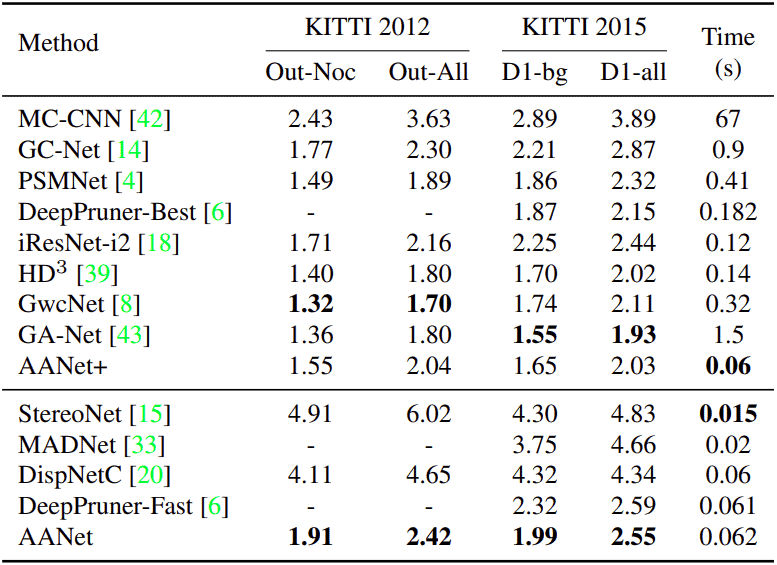
They compare AANet and AANet+ with the counterparts on the SceneFlow (fig. 7) and KITTI (fig. 8) datasets.

results on sceneflow — <strong>Figure 7<strong> Neural networks comparison on SceneFlow dataset

results on kitti depth estimation — <strong>Figure 8<strong> Neural networks comparison on KITTI 2012 and KITTI 2015 datasets

The authors trained models with SceneFlow and KITTI datasets; however, the neural network shows good results on the other domain. For example, you can see the results on the sample from the Middlebury dataset on the fig. 10:

left aloe image — **Figure 9:** Aloe sample from the Middlebury dataset.

right aloe image — **Figure 9:** Aloe sample from the Middlebury dataset.

groundtruth aloe disparity — **Figure 10:** Groundtruth disparity and results of inference of AANet and AANet+.

aloe prediction aanet — **Figure 10:** Groundtruth disparity and results of inference of AANet and AANet+.

Code

The authors provide the code for training, evaluation, and inference in the repository.

LearnOpenCV

Depth Estimation Using Stereo Matching

Classical Approaches For Stereo Matching

Datasets for stereo matching

Deep Learning-Based Approaches for Stereo Matching

AANet