Roadmap To an Automated Image Annotation Tool Using OpenCV Python

Annotation is the most crucial part of a Deep Learning project. It is a deciding factor in how well a model learns. However, it is very tedious and time-consuming. One solution is to use an automated image annotation tool which reduces the time duration greatly.

This article is a part of the pyOpenAnnotate series which includes the following.

1. Roadmap to image annotation using OpenCV.
2. pyOpenAnnotate Workflow.
3. Deploying as a PyPi package.

Here, we will discuss annotation tricks and techniques in OpenCV. These methods will be used to build the automated annotation tool for single class labelling.

• Why Build A Custom Annotation Tool?
• Image Annotation Tool Using OpenCV
• Basic Image Annotation Workflow in OpenCV
• Code Explanation of Image Annotation Tricks in OpenCV
  1. Grayscale Images
  2. Color Segmentation Based Annotation
  3. RGB Color Space Analysis
  4. HSV Color Space Analysis
• Saving Annotations in Different Formats
• Automated Image Annotation Tool Demo

1. Why Build a Custom Annotation Tool Using OpenCV?

In 2022, many annotation tools have numerous features to speed up annotation. RoboFlow and V7 Labs are good examples that have AI-assisted annotation. However, outsourcing annotation may not be the best choice always for the following reasons.

1. Limited free services. Given the cost involved, these services may not be feasible for all.
2. Since annotation is the largest part of any deep learning project, outsourcing adds a huge overhead in terms of cost.
3. There is also the issue of data privacy.

On the other hand, OpenCV has many advantages which even AI-assisted annotation cannot keep up with. A few of them are,

1. Unlike resource hungry deep learning models, OpenCV requires little computation power.
2. It is significantly faster.
3. Invariant to a number of objects; hence it is good for images with a large number of objects.
4. No subscription or one-time payment is involved. It is totally FREE!

Hence, it is important to explore various possibilities before submitting to external sources. Let’s explore a few example data on which we performed annotations using OpenCV.

2. Image Annotation Tool using OpenCV

It is not necessary to manually annotate a dataset every time. Many times, it can be automated using OpenCV. You may think that OpenCV offers limited functionality and it’s not very practical, but let’s not underestimate it yet.

Know that understanding your dataset is the key. The following example images will give you an idea of how and which datasets can be annotated using OpenCV. We will also show you various tricks that can be used to mask out the objects.

3. Basic Image Annotation Workflow in OpenCV

Contour analysis in OpenCV is a powerful tool. We will use it to estimate bounding boxes around detected contours. However, we should not use the out-of-the-box image directly. First, it has to undergo some pre-processing to mask out the objects.

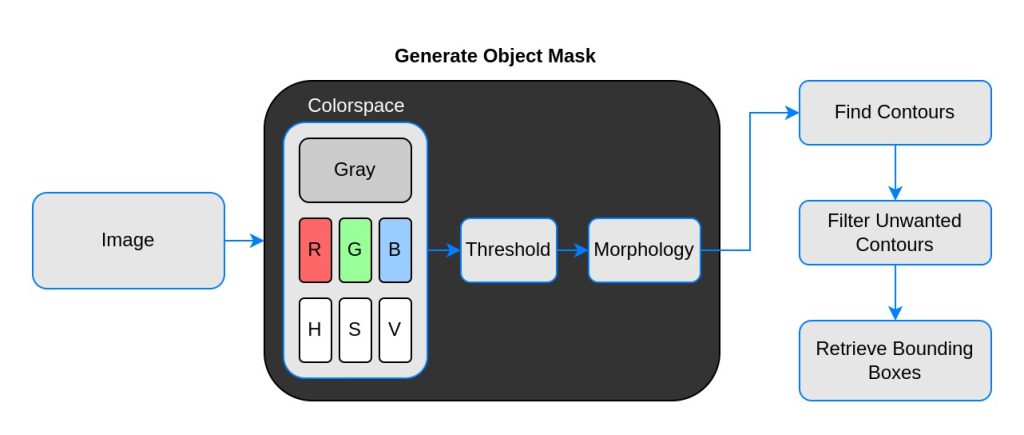
OpenCV reads an image in BGR format by default, whereas thresholding operation accepts only a 1-channel image. We can experiment with different color channels to see which channel is the most contrasting.

Moving forward, thresholding does not guarantee the desired mask always. There will be noises, blobs, edges, etc. To remove these imperfections, morphological operations such as erosion and dilation are applied.

Finally, this 1-channel mask passes through contour analysis to obtain the bounding boxes of the objects. To be specific, top left and bottom right corners. Let’s examine these steps in detail using code.

Click here to download the source code to this post

4. Code Explanation of Image Annotation Tricks in OpenCV

We begin by importing the required libraries, NumPy and OpenCV.

import cv2
import numpy as np
import matplotlib.pyplot as plt
plt.rcParams['image.cmap'] = 'gray'

Load the Images

stags = cv2.imread('stags.jpg')
boars = cv2.imread('boar.jpg')
berries = cv2.imread('strawberries.jpg')
fishes = cv2.imread('fishes.jpg')
coins = cv2.imread('coins.png')
boxes = cv2.imread('boxes2.jpg')

Select Color Space

Let us define a utility function to select the required colorspace. We have added RGB and HSV. The individual channels are stored in a dictionary. Feel free to add more color spaces to experiment with.

def select_colorsp(img, colorsp='gray'):
    # Convert to grayscale.
    gray = cv2.cvtColor(img, cv2.COLOR_BGR2GRAY)
    # Split BGR.
    red, green, blue = cv2.split(img)
    # Convert to HSV.
    im_hsv = cv2.cvtColor(img, cv2.COLOR_BGR2HSV)
    # Split HSV.
    hue, sat, val = cv2.split(im_hsv)
    # Store channels in a dict.
    channels = {'gray':gray, 'red':red, 'green':green, 
                'blue':blue, 'hue':hue, 'sat':sat, 'val':val}
    
    return channels[colorsp]

Utility Function to Display 1×2 Images

The function display() accepts two images and plots side by side. The optional arguments are the titles of the plots, and the figure size,  as shown below.

def display(im_left, im_right, name_l='Left', name_r='Right', figsize=(10,7)):
    
    # Flip channels for display if RGB as matplotlib requires RGB.
    im_l_dis = im_left[...,::-1]  if len(im_left.shape) > 2 else im_left
    im_r_dis = im_right[...,::-1] if len(im_right.shape) > 2 else im_right
    
    plt.figure(figsize=figsize)
    plt.subplot(121); plt.imshow(im_l_dis);
    plt.title(name_l); plt.axis(False);
    plt.subplot(122); plt.imshow(im_r_dis);
    plt.title(name_r); plt.axis(False);

Perform Thresholding

The function thresh() accepts a 1-channel grayscale image. The default threshold value is set to 127. We are performing inverse thresholding as it is more convenient while performing contour analysis. It returns a single-channel thresholded image.

def threshold(img, thresh=127, mode='inverse'):
    im = img.copy()
    
    if mode == 'direct':
        thresh_mode = cv2.THRESH_BINARY
    else:
        thresh_mode = cv2.THRESH_BINARY_INV
    
    ret, thresh = cv2.threshold(im, thresh, 255, thresh_mode)
        
    return thresh

Wondering how to select the perfect threshold value? Use this streamlit app openThreshold to get real-time feedback while thresholding an image.

4.1 Annotation of Infrared Image of Stags

Let’s begin with our first example, infrared images of stags. Our objective is to annotate bounding boxes around the stags as tightly as possible. To recap, we will go through the following steps to mask out the objects (stags in our case). 

1. Select colorspace.
2. Perform thresholding.
3. Perform morphological operations.
4. Contour analysis to find bounding boxes.
5. Filter unnecessary contours.
6. Draw annotations.
7. Save in the required format.

The most important part is to visualize each and every step as you move forward. This will help you make decisions on the next step.

Perform Thresholding on the Appropriate Colorspace

Before performing thresholding operations on any image, it is important to visualize it in different color spaces. We should select the channel with the most contrasting object concerning the background. We will observe this later in another example.

# Select colorspace.
gray_stags = select_colorsp(stags)
# Perform thresholding.
thresh_stags = threshold(gray_stags, thresh=110)


# Display.
display(stags, thresh_stags, 
        name_l='Stags original infrared', 
        name_r='Thresholded Stags',
        figsize=(20,14))

We can see that it is doing a decent job masking the stags. Let’s perform a contour analysis to find bounding boxes around the masks. We have defined a function for the same. We will also define another utility function to draw the bounding boxes.

Perform Contour Analysis to Retrieve Bounding Boxes

The function get_bboxes() accepts a 1-channel image and returns bounding box coordinates of the detected contours. The bounding box coordinates are stored in a tuple in the format (top, left, bottom, right). 

Note that we are sorting and removing the largest contour which is detected around the boundary of the image.

def get_bboxes(img):
    contours, hierarchy = cv2.findContours(img, cv2.RETR_LIST, cv2.CHAIN_APPROX_SIMPLE)
    # Sort according to the area of contours in descending order.
    sorted_cnt = sorted(contours, key=cv2.contourArea, reverse = True)
    # Remove max area, outermost contour.
    sorted_cnt.remove(sorted_cnt[0])
    bboxes = []
    for cnt in sorted_cnt:
        x,y,w,h = cv2.boundingRect(cnt)
        cnt_area = w * h
        bboxes.append((x, y, x+w, y+h))
    return bboxes

Utility Function to Draw Annotations

The function draw_annotation() has two required arguments, the original image, and the bounding box information. Apart from that, you can also set the thickness and color of the boxes using the optional arguments.

def draw_annotations(img, bboxes, thickness=2, color=(0,255,0)):
    annotations = img.copy()
    for box in bboxes:
        tlc = (box[0], box[1])
        brc = (box[2], box[3])
        cv2.rectangle(annotations, tlc, brc, color, thickness, cv2.LINE_AA)
    
    return annotations

As we can see, the stags are being detected, but upon a closer look, there are a few unwanted smaller boxes as well. We will try out the following approaches to resolve this.

• Perform Morphological Operation
• Filter out smaller areas

Refining Detections with Morphological Operations

The function morph_op() is defined to accept a 1-channel image to perform the morphological operation. Select the mode between ‘erosion’, ‘dilation’, ‘open’, and ‘close’. The optional arguments are ksize (kernel size) and number of iterations.

def morph_op(img, mode='open', ksize=5, iterations=1):
    im = img.copy()
    kernel = cv2.getStructuringElement(cv2.MORPH_ELLIPSE,(ksize, ksize))
    
    if mode == 'open':
        morphed = cv2.morphologyEx(im, cv2.MORPH_OPEN, kernel)
    elif mode == 'close':
        morphed = cv2.morphologyEx(im, cv2.MORPH_CLOSE, kernel)
    elif mode == 'erode':
        morphed = cv2.erode(im, kernel)
    else:
        morphed = cv2.dilate(im, kernel)
    
    return morphed

# Perform morphological operation.
morphed_stags = morph_op(thresh_stags)

# Display.
display(thresh_stags, morphed_stags, 
        name_l='Thresholded Stags', 
        name_r='Morphological Operations Result',
        figsize=(20,14))

The results look almost the same! But has it been successful in removing the smaller blobs? Let’s draw the annotations on the morphed stags to find out.

Draw Annotations on Morphed Stags

bboxes = get_bboxes(morphed_stags)
ann_morphed_stags = draw_annotations(stags, bboxes, thickness=5, color=(0,0,255))

# Display.
display(ann_stags, ann_morphed_stags, 
        name_l='Annotating Thresholded Stags', 
        name_r='Annotating Morphed Stags',
        figsize=(20,14))

We can see that the improvement is negligible. Only the blob on the second stag (from left) is gone.

This means that we have to increase the kernel size to take care of the bigger blobs. You can also play around with the number of iterations. However, this will also affect the rest of the image. 

No matter how optimally we set the parameters, some imperfections will always exist. It would be a tedious task to adjust these values when working with thousands of images.

Refining Detections by Filtering Smaller Boxes

In annotation, minuscule bounding boxes have no significant contribution unless we are working with small-scale objects specifically. Let’s complete the pipeline by adding a filtering functionality to the get_bboxes function. By default, we are removing the boxes that are 1000 times smaller than the image. You can adjust this value to work with different images.

def get_filtered_bboxes(img, min_area_ratio=0.001):
    contours, hierarchy = cv2.findContours(img, cv2.RETR_LIST, cv2.CHAIN_APPROX_SIMPLE)
    # Sort the contours according to area, larger to smaller.
    sorted_cnt = sorted(contours, key=cv2.contourArea, reverse = True)
    # Remove max area, outermost contour.
    sorted_cnt.remove(sorted_cnt[0])
    # Container to store filtered bboxes.
    bboxes = []
    # Image area.
    im_area = img.shape[0] * img.shape[1]
    for cnt in sorted_cnt:
        x,y,w,h = cv2.boundingRect(cnt)
        cnt_area = w * h
        # Remove very small detections.
        if cnt_area > min_area_ratio * im_area:
            bboxes.append((x, y, x+w, y+h))
    return bboxes

Draw Annotations After Filtering Small Boxes

bboxes = get_filtered_bboxes(thresh_stags, min_area_ratio=0.001)
filtered_ann_stags = draw_annotations(stags, bboxes, thickness=5, color=(0,0,255))

# Display.
display(ann_stags, filtered_ann_stags, 
        name_l='Annotating Thresholded Stags', 
        name_r='Annotation After Filtering Smaller Boxes',
        figsize=(20,14))

As you can see, we have got the desired result. Now, all we need to do is save the bounding box coordinates in the required format. We will discuss annotation formats in a bit. Let’s look at the results in the full video. Note the crazy FPS!

4.2 Annotating Wild Boars Image

To recap, below are the steps that we followed in the infrared image of stags. We will continue with the same here as well.

• Select color space.
• Perform thresholding.
• Perform morphological operations.
• Find contours and draw annotations.
• Find filtered contours and draw annotations.

Select Color Space and Threshold

# Select color space.
gray_boars = select_colorsp(boars, colorsp='gray')

# Perform thresholding.
thresh_boars = threshold(gray_boars, thresh=140)

# Display.
display(boars, thresh_boars, 
        name_l='Boars Original Infrared', 
        name_r='Thresholded Boars',
        figsize=(20, 14))

Perform Morphological Operation

We can see that the thresholded image has a significantly larger number of white dots. Let’s remove them with morphological operations. Open mode with kernel_size=13 seems to be working perfectly.

# Perform morphological operations.
morph_boars = morph_op(thresh_boars, mode='open', ksize=13)

display(thresh_boars, morph_boars,
        name_l='Thresholded Boars', 
        name_r='Morphed Boars',
        figsize=(20, 14))

Get Filtered Contours and Draw Annotations

# Find contours and draw annotations.
bboxes = get_filtered_bboxes(morph_boars)
# Draw annotations.
ann_boars = draw_annotations(boars, bboxes, thickness=4)

display(boars, ann_boars,
        name_l='Original Boars Infrared', 
        name_r='Annotated Boars',
        figsize=(20, 14))

As you can see, the detections are decent except when the objects are overlapping. This is a limitation of contour detection. We will see how to fix that in a bit.

4.3 Color Segmentation Based Annotation

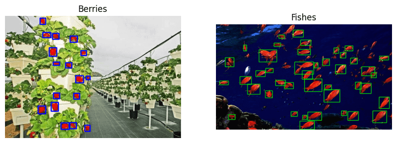
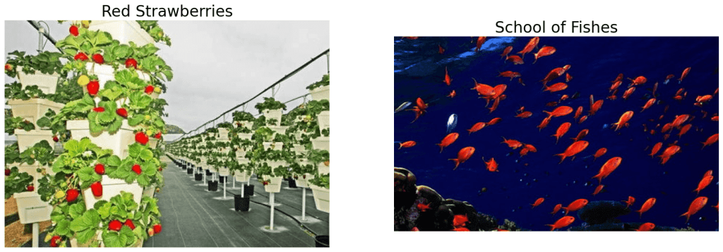
If your dataset has specific colored objects, then color segmentation is the best way to go. We will use the following images – strawberries and fish for demonstration. The objective is to annotate the ripe strawberries and the red school of fish.

Steps to be followed:

1. Pick a color. We will use hsv color space here.
2. Find the color mask.
3. Perform thresholding and morphological operations.
4. Perform contour analysis.
5. Draw annotations.

display(berries, fishes,
       name_l='Red Strawberries',
       name_r='School of Fishes',
       figsize=(20,14))

Generate Color Mask

The function get_colormask() accepts an RGB image along with the range of HSV color values. The keyword arguments lower and upper represent lower and upper HSV boundaries.  It returns a mask using the OpenCV function inRange.

def get_color_mask(img, lower=[0,0,0], upper=[0,255,255]):
    img_hsv = cv2.cvtColor(img, cv2.COLOR_BGR2HSV)
    low = np.array(lower)
    up = np.array(upper)
    mask = cv2.inRange(img_hsv, low, up)
    inv_mask = 255 - mask
    
    return inv_mask

Thresholding and Morphological Operations

mask_berries = get_color_mask(berries, 
                              lower=[0, 211, 111], 
                              upper=[16, 255,255])

# Morphological operation, default is 'open'.
morphed_berries = morph_op(mask_berries)

The above boundaries have been set to mask the red color strawberries. How do we get that? You can either go crazy trying ²²⁵C₆ combinations or find peace using the streamlit app openSegment which is super simple. Adjust the sliders to mask out the desired colors.

Perform Contour Analysis and Draw Annotations

# Contour analysis.
bboxes = get_filtered_bboxes(morphed_berries, 
                             min_area_ratio=0.0005)

# Draw annotations.
ann_berries = draw_annotations(berries, bboxes, 
                               thickness=2, 
                               color=(255,0,0))

# Display.
display(berries, ann_berries,
        name_l='Strawberries', 
        name_r='Annotated Strawberries',
        figsize=(20, 14))

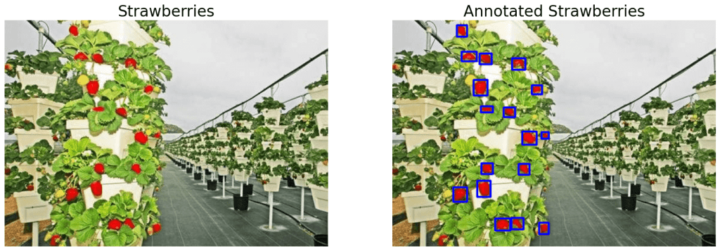
The results look promising. Now you can easily annotate thousands of strawberry images with minimal manual intervention. How about building a strawberry picking robot?

Moving on, let’s try the same approach on the other image with a red school of fish. First, we masked the fishes using the streamlit app openSegment to get the upper and lower HSV boundaries.

# Get the color mask.
mask_fishes = get_color_mask(fishes, 
                             lower=[0, 159, 100], 
                             upper=[71, 255, 255])

# Perform morphological operation, default is 'open'.
morphed_fishes = morph_op(mask_fishes, mode='open')
# Get bounding boxes.
bboxes = get_filtered_bboxes(morphed_fishes)
# Draw annotations.
ann_fishes = draw_annotations(fishes, bboxes, thickness=1)

# Display.
display(fishes, ann_fishes,
        name_l='Fishes', 
        name_r='Annotated Fishes',
        figsize=(20, 14))

4.4 RGB Color Space Analysis

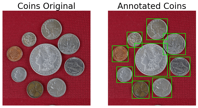
As mentioned earlier, the more the contrast, the better the thresholding. Hence, sometimes it is better to perform thresholding on different channels. Let us take the coin example to understand it better.

Select Color Space

We will use the function select_colorsp() to get the individual color channels.

blue = select_colorsp(coins, colorsp='blue')
green = select_colorsp(coins, colorsp='green')
red = select_colorsp(coins, colorsp='red')
gray = select_colorsp(coins, colorsp='gray')

# Display.
plt.figure(figsize=(20,14))
plt.subplot(141); plt.imshow(blue);
plt.title('Blue'); plt.axis(False);
plt.subplot(142); plt.imshow(green);
plt.title('Green'); plt.axis(False);
plt.subplot(143); plt.imshow(red);
plt.title('Red'); plt.axis(False);
plt.subplot(144); plt.imshow(gray);
plt.title('Gray'); plt.axis(False);

Perform Thresholding

We are using value thresh=74 in this case. Similar to the above examples, it was obtained using openThreshold.

blue_thresh  = threshold(blue,  thresh=74)
green_thresh = threshold(green, thresh=74)
red_thresh   = threshold(red,   thresh=74)
gray_thresh  = threshold(gray,  thresh=74)

# Display.
plt.figure(figsize=(20,14))
plt.subplot(141); plt.imshow(blue_thresh);
plt.title('Blue Threshold'); plt.axis(False);
plt.subplot(142); plt.imshow(green_thresh);
plt.title('Green Threshold'); plt.axis(False);
plt.subplot(143); plt.imshow(red_thresh);
plt.title('Red Threshold'); plt.axis(False);
plt.subplot(144); plt.imshow(gray_thresh);
plt.title('Gray Threshold'); plt.axis(False);

It is clear that thresholding is performing much better on the Green Channel. Let’s continue with the default settings for the thresholded Green Channel.

Morphological Operation, Contour Analysis, and Draw Annotations

# Perform morphological operation.
morph_coin = morph_op(green_thresh)
# Get bounding boxes.
bboxes = get_filtered_bboxes(morph_coin)
# Draw annotations.
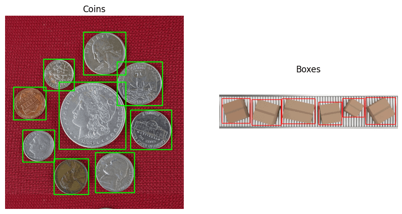
ann_coins = draw_annotations(coins, bboxes)

# Display.
display(coins, ann_coins, 
        name_l='Coins Original', 
        name_r='Annotated Coins', 
        figsize=(10,6))

4.5 HSV Color Space Analysis

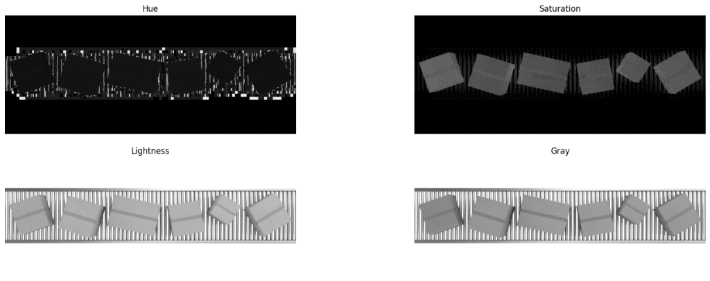
Many times, RGB color space would not be able to separate the required objects as we need. In that case, we can experiment with the other color spaces. An interesting use case of HSV colorspace is shown in the following example of boxes on a rolling conveyor.

Let’s check the individual RGB channels of the box image first.

Inspect RGB Channels

# RGB colorspace.
blue_boxes = select_colorsp(boxes, colorsp='blue')
green_boxes = select_colorsp(boxes, colorsp='green')
red_boxes = select_colorsp(boxes, colorsp='red')
gray_boxes = select_colorsp(boxes, colorsp='gray')

# Display.
plt.figure(figsize=(20,7))
plt.subplot(221); plt.imshow(blue_boxes);
plt.title('Blue'); plt.axis(False);
plt.subplot(222); plt.imshow(green_boxes);
plt.title('Green'); plt.axis(False);
plt.subplot(223); plt.imshow(red_boxes);
plt.title('Red'); plt.axis(False);
plt.subplot(224); plt.imshow(gray_boxes);
plt.title('Gray'); plt.axis(False);

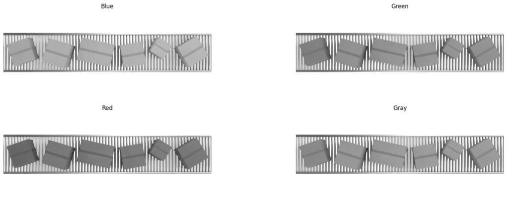
We can see that neither of R, G, B or Gray channels are contrasting. Let’s try with HSV color space.

Inspect HSV Channels

# HSV colorspace.
hue_boxes = select_colorsp(boxes, colorsp='hue')
sat_boxes = select_colorsp(boxes, colorsp='sat')
val_boxes = select_colorsp(boxes, colorsp='val')

# Display.
plt.figure(figsize=(20,7))
plt.subplot(221); plt.imshow(hue_boxes);
plt.title('Hue'); plt.axis(False);
plt.subplot(222); plt.imshow(sat_boxes);
plt.title('Saturation'); plt.axis(False);
plt.subplot(223); plt.imshow(val_boxes);
plt.title('Lightness'); plt.axis(False);
plt.subplot(224); plt.imshow(gray_boxes);
plt.title('Gray'); plt.axis(False);

Annotate The Boxes

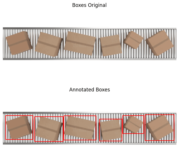
Here it turns interesting. The saturation layer has well contrasting boxes. All we need to do is threshold the saturation layer and perform contour analysis.  Again, we have used the streamlit app openThreshold to arrive at the threshold value (thresh=70) for masking out the objects.

boxes_thresh = threshold(sat_boxes, thresh=70)
morphed_boxes = morph_op(boxes_thresh, mode='open')
bboxes = get_filtered_bboxes(morphed_boxes)
ann_boxes = draw_annotations(boxes, bboxes, thickness=4, color=(0,0,255))

plt.figure(figsize=(10, 7))
plt.subplot(211); plt.imshow(boxes[...,::-1]); 
plt.title('Boxes Original'); plt.axis(False);
plt.subplot(212); plt.imshow(ann_boxes[...,::-1]); 
plt.title('Annotated Boxes'); plt.axis(False);

5. Saving the Annotations in Different Formats

Pascal VOC, YOLO, and COCO are three popular annotation formats used in object detection. Let’s study their structures.

5.1 Pascal VOC

Pascal VOC stores annotations in XML format and looks like the following.

<annotation>
 <folder>Folder_Name</folder>
 <filename>image.jpg</filename>
 <path>PATH_TO_THE_IMAGE</path>
 <size>
  <width>800</width>
  <height>598</height>
  <depth>3</depth>
 </size>
 <object>
  <name>cow</name>
  <bndbox>
   <xmin>40</xmin>
   <ymin>90</ymin>
   <xmax>100</xmax>
   <ymax>350</ymax>
  </bndbox>
 </object>
</annotation>

5.2 YOLO

YOLO annotations are saved in a text file. For each bounding box, it looks like the following. The values are normalized with respect to the height and width of the image.

0 0.0123 0.2345 0.123 0.754

<object-class> <x_centre_norm> <y_centre_norm> <box_width_norm> <box_height_norm>

Let the top left and bottom right coordinates of a bounding box be represented as (x1, y1), and (x2, y2). Then,

x_centre = int ((x2 - x1) / 2)
y_centre = int ((y2 - y1) / 2)

x_centre_norm = x_centre / image_width
y_centre_norm = y_centre / image_height

box_width_norm  = (x2  - x1) / image_width
box_height_norm = (x2  - x1) / image_height

5.3 MS COCO

annotation{
 "id": int,
 "image_id": int,
 "category_id": int, 
 "bbox": [x, y, width, height],
}
categories[{
 "id": int,
 "name": str, 
 "supercategory":str,
}]

5.4 Saving Annotations

There is no hard and fast rule for annotation formats. You would find several more formats being used on various other platforms. Let us save the annotations in YOLO darknet format as an example. You can however modify the function to save in any other format as you please.

def save_annotations(img, bboxes):
    img_height = img.shape[0]
    img_width = img.shape[1]
    with open('image.txt', 'w') as f:
        for box in boxes:
            x1, y1 = box[0], box[1]
            x2, y2 = box[2], box[3]
            
            if x1 > x2:
                x1, x2 = x2, x1
            if y1 > y2:
                y1, y2 = y2, y1
                
            width = x2 - x1
            height = y2 - y1
            x_centre, y_centre = int(width/2), int(height/2)

            norm_xc = x_centre/img_width
            norm_yc = y_centre/img_height
            norm_width = width/img_width
            norm_height = height/img_height

            yolo_annotations = ['0', ' ' + str(norm_xc), 
                                ' ' + str(norm_yc), 
                                ' ' + str(norm_width), 
                                ' ' + str(norm_height), '\n']
            
            f.writelines(yolo_annotations)

6. Automated Image Annotation Tool Demo

Annotation using OpenCV is not perfect. The biggest disadvantage is that it cannot differentiate between classes. Using a contour based approach would select objects irrespective of the class. Moreover, when there are overlapping boundaries, two or more objects can be annotated as one.

We have developed the GUI-based annotation tool pyOpenAnnotate to solve the above mentioned limitation. It uses various techniques we have discussed above to extract foreground masks. 

If the outputs have imperfections, wrong class labelling, or unwanted annotations, those can be removed with a double click. Missing annotations can also be drawn manually.

Conclusion

That’s all about the roadmap to building an Automated Image Annotation Tool using OpenCV. We explored various techniques to localize bounding boxes around objects. To recap, the following are the steps involved.

1. Select the appropriate color space
2. Perform thresholding
3. Perform morphological operations for smoothening
4. Perform contour analysis
5. Filter out unwanted contours
6. Get bounding boxes and draw contours
7. Save detections in various formats

For the past couple of months, we have been working on pyOpenAnnotate. The objective is to build an automated single-class annotation tool using OpenCV. A pip package of the same will be released soon. During the course of this series on annotation, our next article will be on how we built pyOpenAnnotate. It will provide an overall idea of building annotation pipelines.

[Update: Dec 13, 2022]

We have released pyOpenAnnotate pre-Alpha. Install from PYPI using pip install pyOpenAnnotate command. You can find usage instruction in PYPI.

Must Read Articles

References