3D U-Net, a powerful deep learning architecture for medical image segmentation, is designed to process 3D volumetric data like brain tumors, enabling a more comprehensive and precise analysis of brain scans.
In many parts of the world, particularly in the African belt, having access to proper healthcare is a luxury even in 2024. The NCBI report states that, in countries like Uganda the doctor-patient and nurse-patient ratio is approximately 1:25000 and 1:11000 respectively. This is way below the WHO’s recommended doctor-patient ratio of 1:1000 [Source]. This discrepancy poses a significant challenge often hindering timely diagnosis and treatment where the patient has to wait weeks or months for scan results delaying critical post tumor medication and interventions.This is where deep learning based solutions with models like 3D U-Net specialized for volumetric medical images offer a game-changing approach.
In this guide, we will explore how to train a 3D U-Net model from scratch for brain tumor segmentation as part of a BraTS medical AI challenge. With continued efforts from deep learning community and researchers, AI is revolutionizing early stage tumor detection and democratizing access to quality clinical provisions. For the underserved population this could mean a lifeline, reducing wait times, lowering costs and accurate diagnosis of malignant tumors in critical brain regions, potentially saving many lives.
This article is most useful to Kaggle experts, researchers and enthusiasts on lookout for an exciting challenge in the medical domain to extend their expertise for a life saving cause.
- BraTS Annual Challenge
- Glioma: The Hard Problem
- Understanding the Dataset
- Insights from “3D U-Net: Learning Dense Volumetric Segmentation from Sparse Annotation” Paper
- Proposed 3D U-Net Model from Paper
- Code Walkthrough
- Visualize 3D Predictions as Slices using Trained 3D U-Net
- Failure Cases – Not good Predictions
- Key Takeaways
- Conclusion
- References
What is BraTS Annual Challenge all about?

The Brain Tumor Segmentation (BraTS), is an annual challenge presented at the MICCAI (Medical Image Computing and Computer Assisted Intervention) conference. Since 2012, for over a decade now, BraTS competition aims to make use of advanced state of the art deep learning models and techniques to segment lesion regions for early pathological feature detection in brain scans. In regions like Sub-Saharan African (SSA), low-quality technology is often used to capture MRI scans which results in poor image contrast and resolution making it difficult to diagnose. Expert healthcare professionals (especially neuro oncologists and histopathologists) in regions like SSA are limited.
To address the underlying challenges specific to these cases, the BraTS 2023 challenge welcomes individuals and researchers to detect brain tumors in brain scans of patients from African regions on tasks like glioma, pediatric enema, and radiotherapy meningioma.
“ML algorithms for assessment of tumor burden and treatment response based on tumor segmentation on brain MRI were recently shown to BraTS-Africa 2023 Challenge outperform human readers in a large multi-center study of glioma patients. More importantly ML can close survival disparity gaps by overcoming challenges in low-resourced setting, where time consuming manual evaluations are limited to the rare centers in urban areas that can afford highly skilled expert personnel to perform tumor analysis”.
– Page 2, BraTS 2023 paper
Glioma: The Hard Problem
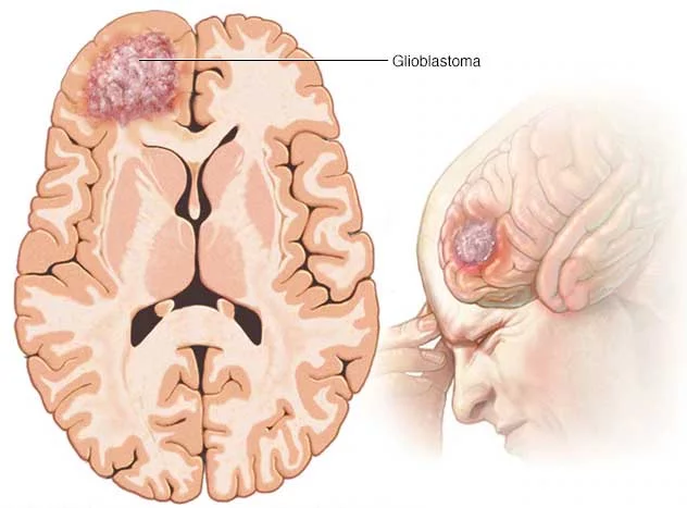
Source httpsaltairhealthcomglasser centerglioblastoma multiforme
Gliomas are malignant types of brain tumors originating from the glial cells that support the brain’s neurons.
These tumors are challenging to diagnose, hard to treat due to, blood-brain barrier, a natural defense mechanism meant to protect the brain from harmful substances, unfortunately blocks the medicinal drugs reaching the brain regions beyond this barrier.
Typically glioma affects the delicate nearby healthy brain tissues making it hard to differentiate between tumor cells and normal tissue. All of these challenges make it one of the deadliest types of cancer with a survival rate of less than 2 years post diagnosis.
Understanding the BraTS2023 Dataset
The semi – automated annotations of BraTS dataset follows a publicly accessible automated pipeline at first, which is then refined in multiple stages by expert neuroradiologists.
The mpMRI scans (multi-parametric) for GLI subset of the BraTS-Africa 2023 challenge are multiple image volumes under different camera settings such as,
1) Native T1-weighted (T1),
2) post gadolinium (Gd) contrast T1-weighted (T1Gd),
3) T2-weighted (T2), and
4) T2 Fluid Attenuated Inversion Recovery (T2-FLAIR).
The dataset consists the following four classes or subregions,
- Class 0: Background / Unlabelled
- Class 1: Necrotic Tumor Core
- Class 2: Peritumoral Edematous/ Invaded Tissue
- Class 3: GD-Enhancing Tumor
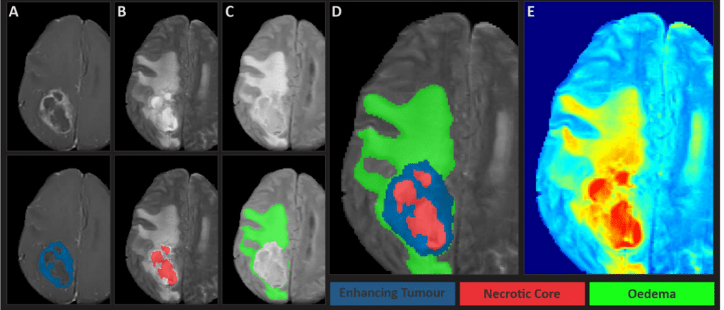
One can access the dataset officially by applying in the synapse project page. For this particular training experiment we will use a subset of BraTS2023-GLI having 625 files from Kaggle. Each volumetric file (.nii) is of (240, 240, 155) dimension.
Here is a link to an interesting anecdote by Satya Mallick where he shares insights from his recent consulting project emphasizing the importance of data understanding. [Link]
Insights from “3D U-Net: Learning Dense Volumetric Segmentation from Sparse Annotation” Paper
We know that usually medical images like MRI and CT scans are high-res and 3D in nature. Annotating these volumetric data slice by slice is tedious and time-consuming. This approach is also inefficient, as neighboring slices often contain similar information. So ideally an optimal approach would be to annotate slices sparsely. From these sparse annotations the network learns underlying features and predicts dense 3D segments.
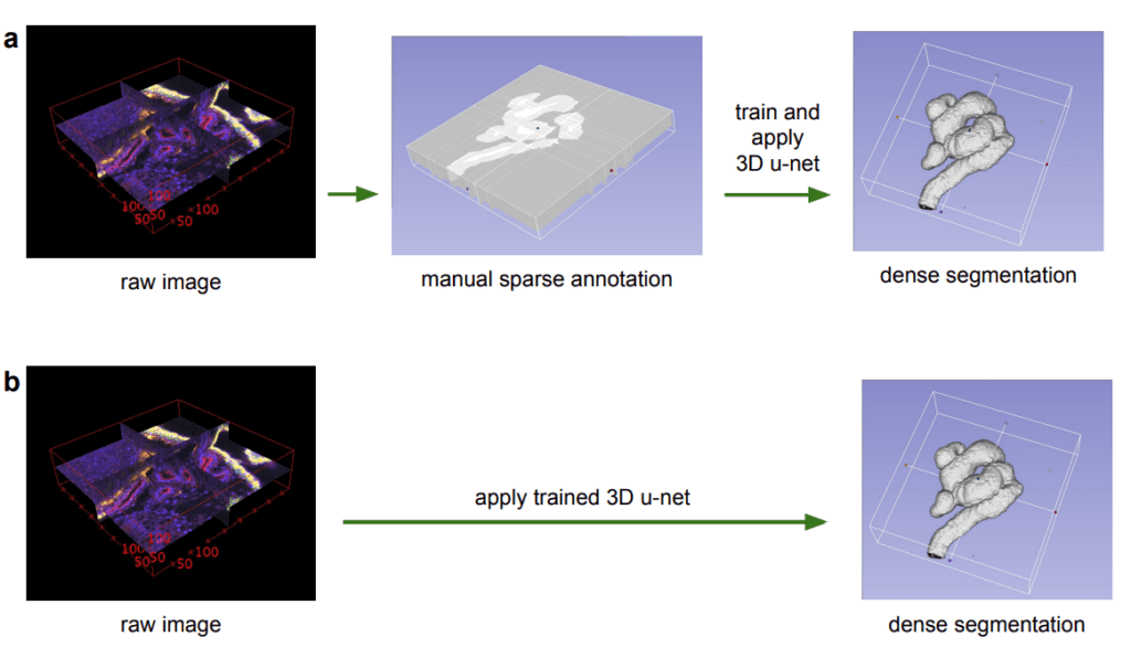
The paper proposes 3D U-Net, an extension of traditional U-Net incorporating 3D Convolutions for processing volumetric data. In 3D Convolutions, a 3D kernel is applied to extract feature representations across three dimensions. They have advantage in scenarios where the additional dimension (C,D,H,W) such as temporal aspect (e.g. time) in videos or depth (D) in medical images are invaluable.
But you may wonder why we need to increase the complexity when we can train a simple 2D U-Net by processing volumes slice by slice?
While it’s a reasonable approach, a 2D Convolutions may fail to capture the rich contextual information and spatial patterns that’s available across the slices which is crucial in brain tumor segmentation. Typically tumors are not confined to a single slice, they spread across the slices. If they are processed independently, this leads to loss in information about the overall structure of the mass and leads to suboptimal segmentation.
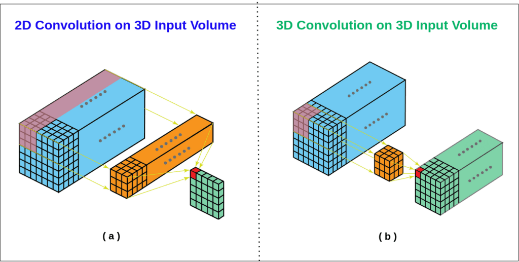
Source httpsaistackexchangecomquestions13692when should i use 3d convolutions
In contrast, 3D Convolutions can attend to multi plane slices simultaneously and extract intricate spatial relationships between neighboring slices enabling much more accurate segmentation.
Proposed 3D U-Net Model from Paper
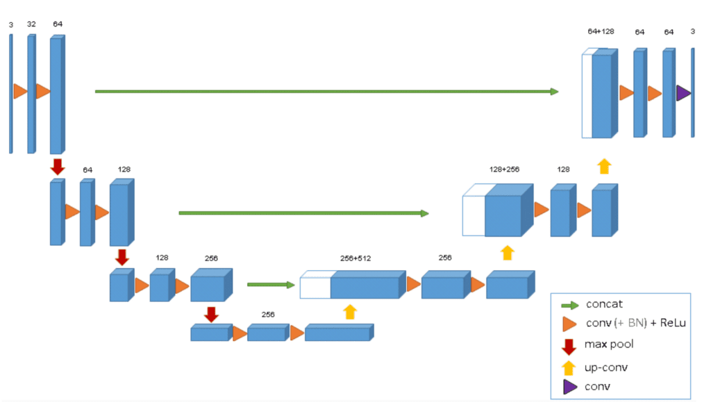
The 3D paper discusses the use of the BatchNorm layer within the ConvNet for faster convergence and setting zero weights for unlabeled pixels to generalize the whole volume. Keeping these model configurations as reference we will define a 3D U-Net mode similar to this, in the upcoming code section.
The following table from the paper reports the quantified differences in IoU metrics between 3D U-Net and 2D U-Net for volumetric data. We can clearly see that 3D U-Net has a significant boost in metrics compared to 2D U-Net across all test volumes.
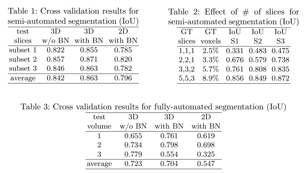
Now, we got a good hold why 3D U-Net is suitable for volumetric data. Let’s jump directly into the implementation to spin up our experiments.
Code Walkthrough of Training a 3D U-Net
Installing Dependencies
Our dataset files are in neuroimaging (.nii) file format. We will use the nibabel library to efficiently read and manipulate these 3D brain volumes. For loss functions and metric evaluation of 3D segmentation tasks, segmentation-models-pytorch-3d package comes handy, which lets us to focus on other essential parts like understanding the dataset and model preparation.
!pip install nibabel -q
!pip install scikit-learn -q
!pip install tqdm -q
!pip install split-folders -q
!pip install torchinfo -q
!pip install segmentation-models-pytorch-3d -q
!pip install livelossplot -q
!pip install torchmetrics -q
!pip install tensorboard -q
Now let’s import some key modules that we will use throughout the training pipeline.
import os
import random
import splitfolders
from tqdm import tqdm
import nibabel as nib
import glob
import numpy as np
import matplotlib.pyplot as plt
from sklearn.preprocessing import MinMaxScaler
from sklearn.model_selection import train_test_split
import shutil
import time

from dataclasses import dataclass

import torch
import torch.nn as nn
import torch.nn.functional as F
from torch.optim import Adam
from torch.optim.lr_scheduler import CosineAnnealingLR
import torchvision.transforms as transforms
from torch.cuda import amp

from torchmetrics import MeanMetric
from torchmetrics.classification import MulticlassAccuracy

from torch.utils.data import Dataset, DataLoader
from torch.utils.tensorboard import SummaryWriter
from torchinfo import summary
import gc

import segmentation_models_pytorch_3d as smp

from livelossplot import PlotLosses
from livelossplot.outputs import MatplotlibPlot, ExtremaPrinter
The following code snippets is to download the dataset and unzip it in a specified directory.
!pip install kaggle -q
!kaggle datasets download -d aiocta/brats2023-part-1
Note: The subset we will download is 7GB in size (compressed). When the dataset is extracted it almost occupies tenfolds (76.82 GB) disk space. We will delete the raw data files immediately after unzipping and preprocessing them to save only the ROI crops thereby saving disk space.
!sudo apt install unzip
!unzip brats2023-part-1.zip -d BraTS2023-Glioma/
!rm -rf workspace/brats2023-part-1.zip
Set seeds for reproducibility.
def seed_everything(SEED):
   np.random.seed(SEED)
   torch.manual_seed(SEED)
   torch.cuda.manual_seed_all(SEED)
   torch.backends.cudnn.deterministic = True
   torch.backends.cudnn.benchmark = False


def get_default_device():
   gpu_available = torch.cuda.is_available()
   return torch.device('cuda' if gpu_available else 'cpu'), gpu_available
For readability, we will store hyperparameters within a TrainingConfig dataclass. The hardware config for training was i7, 64GB RAM, 12 GB vRAM, and 24 cpu cores . To converge to a relatively minimal loss within less epochs, we will use 1e-3, for 100 epochs and a batch size of 5 is chosen to fit it to the GPU being used.
@dataclass(frozen=True)
class TrainingConfig:
   BATCH_SIZE:      int = 5
   EPOCHS:          int = 100
   LEARNING_RATE: float = 1e-3
   CHECKPOINT_DIR:  str = os.path.join('model_checkpoint', '3D_UNet_Brats2023')
   NUM_WORKERS:     int = 4
Sample Preprocessing
scaler = MinMaxScaler()

DATASET_PATH = "BraTS2023-Glioma"
print("Total Files: ", len(os.listdir(DATASET_PATH)))
Total Files:  625
Each folder within the data root directory will have multiple volumes and subdirectories will have the following files structure.
!tree -L 2 BraTS2023-Glioma/BraTS-GLI-00000-000

BraTS2023-Glioma/BraTS-GLI-00000-000
├── BraTS-GLI-00000-000-seg.nii
├── BraTS-GLI-00000-000-t1c.nii
├── BraTS-GLI-00000-000-t1n.nii
├── BraTS-GLI-00000-000-t2f.nii
└── BraTS-GLI-00000-000-t2w.nii
Load the NifTI image using nib.load() which returns a numpy array.
# Load the NIfTI image
sample_image_flair = nib.load(os.path.join(DATASET_PATH , "BraTS-GLI-00000-000/BraTS-GLI-00000-000-t2f.nii")).get_fdata()
print("Original max value:", sample_image_flair.max())
# Original max value: 2934.0

# Reshape the 3D image to 2D for scaling
sample_image_flair_flat = sample_image_flair.reshape(-1, 1)
We will use MinMaxScaler(), to scale the pixel values within 0 to 1 which helps the values to follow a normal distribution. For better understanding about the volumes (.nii), we will take a sample and perform all the preprocessing that we are going to perform on the entire dataset.
# Apply scaling
sample_image_flair_scaled = scaler.fit_transform(sample_image_flair_flat)

# Reshape it back to the original 3D shape
sample_image_flair_scaled = sample_image_flair_scaled.reshape(sample_image_flair.shape)

print("Scaled max value:", sample_image_flair_scaled.max())
print("Shape of scaled Image: ", sample_image_flair_scaled.shape)

#Scaled max value: 1.0
#Shape of scaled Image:  (240, 240, 155)
Similarly other sequences, t1, t1ce, t2 will have pixel range of [0, 1] and (240, 240, 155) image dimensions after scaling with scaler.fit_transform( ).
Along these MRI modalities, a binary mask of shape (240, 240, 155) with different gray intensities exists. We will simply convert its precision to unsigned int to have intensity value between 0 and 255.
sample_mask = nib.load(
    DATASET_PATH + "/BraTS-GLI-00000-000/BraTS-GLI-00000-000-seg.nii"
).get_fdata()
sample_mask = sample_mask.astype(np.uint8)  # values between 0 and 255

print("Unique class in the mask", np.unique(sample_mask))
# Unique class in the mask [0 1 2 3]
# Shape of mask:  (240, 240, 155)
Let’s choose a random slice and visualize it per modality for better insights on how the data and mask looks like. Before training any deep learning model it is crucial to understand what your dataset speaks.
n_slice = random.randint(0, sample_mask.shape[2])  # random slice between 0 - 154

plt.figure(figsize = (12,8))

plt.subplot(231)
plt.imshow(sample_image_flair_scaled[:,:,n_slice], cmap='gray')
plt.title('Image flair')

plt.subplot(232)
plt.imshow(sample_image_t1[:,:,n_slice], cmap = "gray")
plt.title("Image t1")

plt.subplot(233)
plt.imshow(sample_image_t1ce[:,:,n_slice], cmap='gray')
plt.title("Image t1ce")

plt.subplot(234)
plt.imshow(sample_image_t2[:,:,n_slice], cmap = 'gray')
plt.title("Image t2")

plt.subplot(235)
plt.imshow(sample_mask[:,:,n_slice])
plt.title("Seg Mask")

plt.subplot(236)
plt.imshow(sample_mask[:,:,n_slice], cmap = 'gray')
plt.title('Mask Gray')
plt.show()
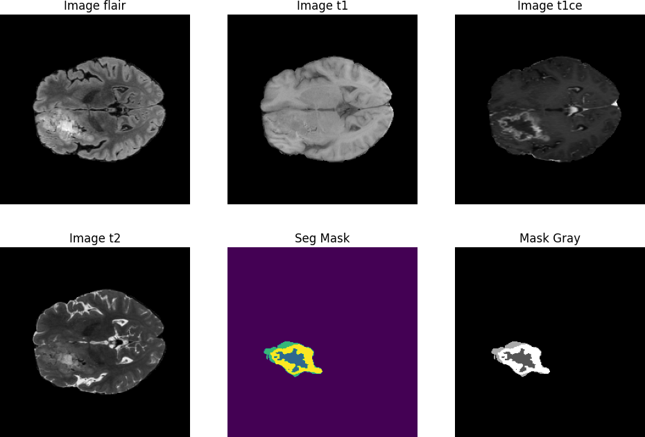
Based on the observations and community suggestions, instead of training each modality individually, we can stack them into a single sequence along the last dimension. This gives a combined representation of rich information available across modalities about the entire brain scan.
combined_x = np.stack(
    [sample_image_flair_scaled, sample_image_t1ce, sample_image_t2], axis=3
)  # along the last channel dimension.
print("Shape of Combined x ", combined_x.shape)
# Shape of Combined x  (240, 240, 155, 3)
Training the whole dataset with original image dimensions would be memory intensive and is not necessary. Therefore, an optimal approach to consider only the ROI. (i.e. around the brain region). Through trial and error, slicing and cropping the area approximately between 56 and 184 has been found to be a more appropriate ROI.
combined_x = combined_x[56:184, 56:184, 13:141]
print("Shape after cropping: ", combined_x.shape)

sample_mask_c = sample_mask[56:184,56:184, 13:141]
print("Mask shape after cropping: ", sample_mask_c.shape)

#Shape after cropping:  (128, 128, 128, 3)
#Mask shape after cropping:  (128, 128, 128)
Coming to ground truth mask preprocessing, as usual multi-class semantic segmentation task, we can convert the numpy mask into one hot encoded tensor of int64 dtype for each pixel in the image. One hot encoding expects the mask to be in integer format for categorical values. For eg: If a mask contains class 0 and class 1, one hot encode would look like [1,0,1,0].
sample_mask_cat  = F.one_hot(torch.tensor(sample_mask_c, dtype = torch.long), num_classes = 4)

#0,1,2,3  -> dtype = torch.long as F.one_hot expects in int64
Ok, now we understood all the necessary preprocessing steps to be performed with a single sample. Next we will move on applying the same logic for all the files.
t1ce_list = sorted(glob.glob(f"{DATASET_PATH}/*/*t1c.nii"))
t2_list = sorted(glob.glob(f"{DATASET_PATH}/*/*t2w.nii"))
flair_list = sorted(glob.glob(f"{DATASET_PATH}/*/*t2f.nii"))
mask_list = sorted(glob.glob(f"{DATASET_PATH}/*/*seg.nii"))

print("t1ce list: ", len(t1ce_list))
print("t2 list: ", len(t2_list))
print("flair list: ", len(flair_list))
print("Mask list: ", len(mask_list))
#t1ce list:  625
#t2 list:  625
#flair list:  625
#Mask list:  625
Dataset Preprocessing
The following loop iterates over all the files from different MRI modalities, stack them into multi-channel format along the last dimension and save them as a .npy file. Here np.unqiue() returns the unique class values and their corresponding counts of a segmentation mask.
To optimize computation, we can flexibly ignore or skip image volumes that contain less than 1% non-background pixels. This strategy reduces the computation overhead without sacrificing important features.
for idx in tqdm(
    range(len(t2_list)), desc="Preparing to stack, crop and save", unit="file"
):
    temp_image_t1ce = nib.load(t1ce_list[idx]).get_fdata()
    temp_image_t1ce = scaler.fit_transform(
        temp_image_t1ce.reshape(-1, temp_image_t1ce.shape[-1])
    ).reshape(temp_image_t1ce.shape)

    temp_image_t2 = nib.load(t2_list[idx]).get_fdata()
    temp_image_t2 = scaler.fit_transform(
        temp_image_t2.reshape(-1, temp_image_t2.shape[-1])
    ).reshape(temp_image_t2.shape)

    temp_image_flair = nib.load(flair_list[idx]).get_fdata()
    temp_image_flair = scaler.fit_transform(
        temp_image_flair.reshape(-1, temp_image_flair.shape[-1])
    ).reshape(temp_image_flair.shape)

    temp_mask = nib.load(mask_list[idx]).get_fdata()

    temp_combined_images = np.stack(
        [temp_image_flair, temp_image_t1ce, temp_image_t2], axis=3
    )

    temp_combined_images = temp_combined_images[56:184, 56:184, 13:141]
    temp_mask = temp_mask[56:184, 56:184, 13:141]

    val, counts = np.unique(temp_mask, return_counts=True)

    # If a volume has less than 1% of mask, we simply ignore to reduce computation
    if (1 - (counts[0] / counts.sum())) > 0.01:
        #         print("Saving Processed Images and Masks")
        temp_mask = F.one_hot(torch.tensor(temp_mask, dtype=torch.long), num_classes=4)
        os.makedirs("BraTS2023_Preprocessed/input_data_3channels/images", exist_ok=True)
        os.makedirs("BraTS2023_Preprocessed/input_data_3channels/masks", exist_ok=True)

        np.save(
            "BraTS2023_Preprocessed/input_data_3channels/images/image_"
            + str(idx)
            + ".npy",
            temp_combined_images,
        )
        np.save(
            "BraTS2023_Preprocessed/input_data_3channels/masks/mask_"
            + str(idx)
            + ".npy",
            temp_mask,
        )

    else:
        pass
After all the processing steps, we are left with 575 total image and mask samples.
images_folder = "BraTS2023_Preprocessed/input_data_3channels/images"
print(len(os.listdir(images_folder)))

masks_folder = "BraTS2023_Preprocessed/input_data_3channels/masks"
print(len(os.listdir(masks_folder)))
# Images: 575
# Masks: 575
Using splitfolders.ratio(), we can split into training and validation samples in separate directories with a test split ratio of 0.25.
input_folder = "BraTS2023_Preprocessed/input_data_3channels/"

output_folder = "BraTS2023_Preprocessed/input_data_128/"

splitfolders.ratio(
    input_folder, output_folder, seed=42, ratio=(0.75, 0.25), group_prefix=None
)
Note: If you are bound with limited storage, after preprocessing, remove the raw (.nii) files which can free disk space of around 77GB.
if os.path.exists(input_folder):
    shutil.rmtree(input_folder)
    print(f"{input_folder} is removed")
else:
    print(f"{input_folder} doesn't exist")
Custom DataLoader
To move onto final dataset preparation, we will define a custom PyTorch Dataset which handles file loading, transformations etc. As usual, the __len__ returns the length of total files in the img_list.
class BratsDataset(Dataset):
    def __init__(self, img_dir, mask_dir, normalization=True):
        super().__init__()

        self.img_dir = img_dir
        self.mask_dir = mask_dir
        self.img_list = sorted(
            os.listdir(img_dir)
        )  # Ensure sorting to match images and masks
        self.mask_list = sorted(os.listdir(mask_dir))
        self.normalization = normalization

        # If normalization is True, set up a normalization transform
        if self.normalization:
            self.normalizer = transforms.Normalize(
                mean=[0.5], std=[0.5]
            )  # Adjust mean and std based on your data

    def load_file(self, filepath):
        return np.load(filepath)

    def __len__(self):
        return len(self.img_list)
Next __getitem__ dunder method is defined which takes in an index( idx) and loads the image and corresponding masks for that index. We will also apply a simple normalization using torch.transforms(). At last this returns the normalized image and mask tensors.
class BraTSDataset(Dataset):
. . .
def __getitem__(self, idx):
       image_path = os.path.join(self.img_dir, self.img_list[idx])
       mask_path = os.path.join(self.mask_dir, self.mask_list[idx])
       # Load the image and mask
       image = self.load_file(image_path)
       mask = self.load_file(mask_path)

       # Convert to torch tensors and permute axes to C, D, H, W format (needed for 3D models)
       image = torch.from_numpy(image).permute(3, 2, 0, 1)  # Shape: C, D, H, W
       mask = torch.from_numpy(mask).permute(3, 2, 0, 1)  # Shape: C, D, H, W

       # Normalize the image if normalization is enabled
       if self.normalization:
           image = self.normalizer(image)

       return image, mask
Now all is set. Let’s initialize the BraTSDataset class and pass the train and val images directory. We will have 431 train and 144 validation dataset samples.
train_img_dir = "BraTS2023_Preprocessed/input_data_128/train/images"
train_mask_dir = "BraTS2023_Preprocessed/input_data_128/train/masks"

val_img_dir = "BraTS2023_Preprocessed/input_data_128/val/images"
val_mask_dir = "BraTS2023_Preprocessed/input_data_128/val/masks"

val_img_list = os.listdir(val_img_dir)
val_mask_list = os.listdir(val_mask_dir)

# Initialize datasets with normalization only
train_dataset = BraTSDataset(train_img_dir, train_mask_dir, normalization=True)
val_dataset = BraTSDataset(val_img_dir, val_mask_dir, normalization=True)

# Print dataset statistics
print("Total Training Samples: ", len(train_dataset))
print("Total Val Samples: ", len(val_dataset))
#Total Training Samples:  431
#Total Val Samples:  144
Using this train and val dataloader are prepared with a batch size of 5 and num_workers = 4.
train_loader = DataLoader(train_dataset, batch_size = 5, shuffle = True, num_workers = 4)
val_loader = DataLoader(val_dataset, batch_size = 5, shuffle = False, num_workers = 4)

#Sanity Check
images, masks = next(iter(train_loader))
print(f"Train Image batch shape: {images.shape}")
print(f"Train Mask batch shape: {masks.shape}")
Train Image batch shape: torch.Size([5, 3, 128, 128, 128])
Train Mask batch shape: torch.Size([5, 4, 128, 128, 128])
To ensure the dataset preparation logic went fine, let’s visualize middle slices of multiple volumes.
def visualize_slices(images, masks, num_slices=20):
    batch_size = images.shape[0]

    masks = torch.argmax(masks, dim=1)  # along the channel/class dim

    for i in range(min(num_slices, batch_size)):
        fig, ax = plt.subplots(1, 5, figsize=(15, 5))

        middle_slice = images.shape[2] // 2
        ax[0].imshow(images[i, 0, middle_slice, :, :], cmap="gray")
        ax[1].imshow(images[i, 1, middle_slice, :, :], cmap="gray")
        ax[2].imshow(images[i, 2, middle_slice, :, :], cmap="gray")
        ax[3].imshow(masks[i, middle_slice, :, :], cmap="viridis")
        ax[4].imshow(masks[i, middle_slice, :, :], cmap="gray")

        ax[0].set_title("T1ce")
        ax[1].set_title("FLAIR")
        ax[2].set_title("T2")
        ax[3].set_title("Seg Mask")
        ax[4].set_title("Mask - Gray")

        plt.show()


visualize_slices(images, masks, num_slices=20)

Ok, we can confirm that everything is perfect about data loader preparation.
Building a 3D U-Net Model : Constructing One Block at a Time
MONAI Model Zoo hosts a suite of medical imaging models including pre-trained checkpoints for the BraTS2018 dataset. You can finetune these models for better metrics and prediction. However in our training pipeline we will build the 3D U-Net model from scratch to get intuitive understanding about the model architecture and its capabilities.
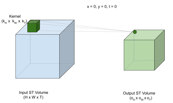
Source httpslivebookmanningcombookmath and architectures of deep learningchapter 10v 10201
Before starting with 3D U-Net, we will define a handy utility (double_conv),which defines two sequential, nn.Conv3D blocks with a 3x3x3 kernel and the same or zero padding is applied.
Same padding ensures that the spatial dimensions of the input image aren’t reduced by the convolution operation. Each Conv3D block is followed by a batch normalization (BatchNorm3d) and ReLU activation (Conv3DNormActivation). Additionally a dropout layer of probability (p = 0.1) is applied for filters that have 32 channels and p = 0.3 applied for filters with 128 channels.
# Define the double_conv function
def double_conv(in_channels, out_channels):
   return nn.Sequential(
       nn.Conv3d(in_channels, out_channels, kernel_size=3, padding=1),
       nn.BatchNorm3d(out_channels),  # Add BatchNorm3d after convolution
       nn.ReLU(inplace=True),
       nn.Dropout(0.1 if out_channels <= 32 else 0.2 if out_channels <= 128 else 0.3),
       nn.Conv3d(out_channels, out_channels, kernel_size=3, padding=1),
       nn.BatchNorm3d(out_channels),  # Add BatchNorm3d after second convolution
       nn.ReLU(inplace=True)
   )
As we discussed earlier, a 3DUNet is simply an extension of the well known 2D U-Net architecture adapted to handle 3D inputs.
Contraction Path or Encoder
- The encoder progressively downsamples the input with the `double_conv()` function defined earlier. Following this a `MaxPool3D` layer is added with a 2x2x2 kernel, which reduces the spatial resolution by a factor of 2.
- The encoder consists of four double_conv blocks. Each block increases the feature map for learning deeper semantic representations while reducing the spatial dimensions by half.
- The output channels increase from in_channels (3 in our case), 16, 32, 64 and 128.
class UNet3D(nn.Module):
   def __init__(self, in_channels, out_channels):
       super().__init__()

       # Contraction path
       self.conv1 = double_conv(in_channels=in_channels, out_channels=16)
       self.pool1 = nn.MaxPool3d(kernel_size=2)

       self.conv2 = double_conv(in_channels=16, out_channels=32)
       self.pool2 = nn.MaxPool3d(kernel_size=2)

       self.conv3 = double_conv(in_channels=32, out_channels=64)
       self.pool3 = nn.MaxPool3d(kernel_size=2)

       self.conv4 = double_conv(in_channels=64, out_channels=128)
       self.pool4 = nn.MaxPool3d(kernel_size=2)
BottleNeck Layer
- Next, the bottleneck layer is defined which is a single double_conv block. In U-Net it is called bottleneck because it is at the lowest point in the U-Net architecture and is the transition point from encoder to decoder.
- The BottleNeck layer will have the highest number of channels in the entire 3D U-Net network, which process the compact representation capturing rich semantic features.
class UNet3D(nn.Module):
   def __init__(self, in_channels, out_channels):
       super().__init__()

	#Encoder
   . . .
	self.conv5 = double_conv(in_channels=128, out_channels=256)
Decoder or Expansive path
The decoder contains several blocks which gradually expand the compressed or high level feature maps after the bottleneck layer, to an output representation that has original input dimensions with bilinear interpolation.
The decoder is comprised of three main stages:
- UpSampling : For upsampling, 3D Transposed Convolutions are used. This reduces the number of filters while increasing the spatial resolution.
- Skip Connections: To combine the low level features in the starting of the network with the high level features during decoder upsampling, the U-Net makes use of skip connections which concatenates the features from previous encoder layers. For this the number of filters has to be matched between the encoder and the upsampled output in the decoder.
- Refinement: After concatenating the features, a double convolution operation is performed which refines the combined features.
Just like encoder, the decoder has four blocks of ConvTranspose3D layer followed by double_conv operation.
Finally a Conv3D operation with 1x1x1 kernel with out_channels = num_classes is employed to map the learned features to output a multi-channel mask which implies each channel corresponds to a predicted class.
class UNet3D(nn.Module):
   def __init__(self, in_channels, out_channels):
       super().__init__()

	#Encoder
   . . .
	#BottleNeck
	self.conv5 = double_conv(in_channels=128, out_channels=256)

	#Decoder or Expansive path
	self.upconv6 = nn.ConvTranspose3d(in_channels=256, out_channels=128, kernel_size=2, stride=2)
       self.conv6 = double_conv(in_channels=256, out_channels=128)

       self.upconv7 = nn.ConvTranspose3d(in_channels=128, out_channels=64, kernel_size=2, stride=2)
       self.conv7 = double_conv(in_channels=128, out_channels=64)

       self.upconv8 = nn.ConvTranspose3d(in_channels=64, out_channels=32, kernel_size=2, stride=2)
       self.conv8 = double_conv(in_channels=64, out_channels=32)

       self.upconv9 = nn.ConvTranspose3d(in_channels=32, out_channels=16, kernel_size=2, stride=2)
       self.conv9 = double_conv(in_channels=32, out_channels=16)


       self.out_conv = nn.Conv3d(in_channels=16, out_channels=out_channels, kernel_size=1)
The following forward method implements all the operations and functionalities discussed earlier for single forward pass through the defined 3D U-Net network.
class UNet3D(nn.Module):
   . . .
    def forward(self, x):
       # Contracting path
       c1 = self.conv1(x)
       p1 = self.pool1(c1)

       c2 = self.conv2(p1)
       p2 = self.pool2(c2)

       c3 = self.conv3(p2)
       p3 = self.pool3(c3)

       c4 = self.conv4(p3)
       p4 = self.pool4(c4)  # downscale

       c5 = self.conv5(p4)

       # Expansive path
       u6 = self.upconv6(c5)  # upscale
       u6 = torch.cat([u6, c4], dim=1)  # skip connections along channel dim
       c6 = self.conv6(u6)

       u7 = self.upconv7(c6)
       u7 = torch.cat([u7, c3], dim=1)
       c7 = self.conv7(u7)

       u8 = self.upconv8(c7)
       u8 = torch.cat([u8, c2], dim=1)
       c8 = self.conv8(u8)

       u9 = self.upconv9(c8)
       u9 = torch.cat([u9, c1], dim=1)
       c9 = self.conv9(u9)

       outputs = self.out_conv(c9)

       return outputs
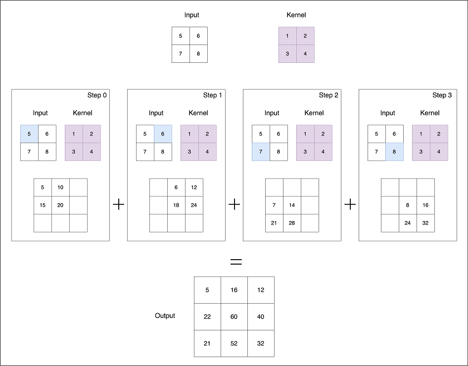
Source httpslivebookmanningcombookmath and architectures of deep learningchapter 10v 10201
Initialize the 3D U-Net model and perform a forward pass with dummy input to verify that we get expected output shape.
# Test the model
model = UNet3D(in_channels=3, out_channels=4)
print(model)

# Create a random input tensor
ip_tensor = torch.randn(1, 3, 128, 128, 128)

# Forward pass through the model
output = model(ip_tensor)

# Print input and output shapes
print("-" * 260)
print(f"Input shape: {ip_tensor.shape}")
print(f"Output shape: {output.shape}")
#Input shape: torch.Size([1, 3, 128, 128, 128])
#Output shape: torch.Size([1, 4, 128, 128, 128])
Defining Losses and Optimizers from Segmentation Models PyTorch
Choosing the right loss function for a given task is a key aspect in any deep learning training. For semantic segmentation tasks, region based losses like Dice+Cross Entropy works well. However if the dataset is heavily imbalanced as in our case, we can combine region based (Dice) and distribution based (Focal) loss functions for optimal convergence. The smp package has some set of predefined loss functions to serve this purpose.
- To prevent NAN values and ensure training stability, a smooth factor of
1e-5is applied within the dice loss function. - To address class imbalance, focal loss is used with a class weighing factor of
0.25, assigning more weights to hard to classify instances with a focussing parameter ofgamma=0.2. - Both of these losses are combined together for balanced convergence.
dice_loss = smp.losses.DiceLoss(
   mode="multiclass",          # For multi-class segmentation
   classes=None,               # Compute the loss for all classes
   log_loss=False,             # Do not use log version of Dice loss
   from_logits=True,           # Model outputs are raw logits
   smooth=1e-5,                # A small smoothing factor for stability
   ignore_index=None,          # Don't ignore any classes
   eps=1e-7                    # Epsilon for numerical stability
)

# Focal Loss with optional class balancing via alpha
focal_loss = smp.losses.FocalLoss(
   mode="multiclass",          # Multi-class segmentation
   alpha=0.25,                 # class weighting to deal with class imbalance
   gamma=2.0                   # Focusing parameter for hard-to-classify examples
)

def combined_loss(output, target):
   loss1 = dice_loss(output, target)
   loss2 = focal_loss(output, target)
   return loss1 + loss2ave
We will need to save checkpoints based on best valid loss, therefore a simple utility function to save the best checkpoints incrementally is defined. In each versioned directory, Tensorboard events file and a ckpt.tar file containing the model.state_dict() and optimizer.state_dict() are saved.
def create_checkpoint_dir(checkpoint_dir):
    if not os.path.exists(checkpoint_dir):
        os.makedirs(checkpoint_dir)
    try:
        num_versions = [
            int(i.split("_")[-1]) for i in os.listdir(checkpoint_dir) if "version" in i
        ]
        version_num = max(num_versions) + 1

    except:
        version_num = 0

    version_dir = os.path.join(checkpoint_dir, "version_" + str(version_num))
    os.makedirs(version_dir)

    print(f"Checkpoint directory: {version_dir}")
    return version_dir
The AdamW optimizer is chosen with a learning rate of 1e-3 and a weight decay of 1e-2 which acts as a regularization step to prevent overfitting by applying L2 norm. In some cases, the adaptive learning rate of Adam might lead to suboptimal convergence which is a known issue. Inorder to prevent instability by this, amsgrad is enabled which ensures learning rate is not increased, thus avoiding large steps during weight update especially in noisy past gradients.
seed_everything(SEED = 42)

DEVICE, GPU_AVAILABLE  = get_default_device()
print(DEVICE)

CKPT_DIR = create_checkpoint_dir(TrainingConfig.CHECKPOINT_DIR)

from torch.optim import AdamW

optimizer = AdamW(
   model.parameters(),
   lr=TrainingConfig.LEARNING_RATE,
   weight_decay=1e-2,                # Regularization to avoid overfitting
   amsgrad=True                      # Optional AMSGrad variant
)
To wrap things up, the train and validate functions are implemented. We selected IoU, a common metric in segmentation tasks to evaluate the overlap between ground truth mask and prediction segmentation. To compute this, smp.metrics.iou_score(tp, fp, fn, tn, reduction= 'macro') is used, where reduction = macro averages IoU across all classes. Additionally, the MulticlassAccuracy metric from Torchmetrics helps to determine the classification accuracy of each pixel, assessing how well the model assigns the correct class label to each pixel.
Training our 3D U-Net model
def train_one_epoch(
   model,
   loader,
   optimizer,
   num_classes,
   device="cpu",
   epoch_idx=800,
   total_epochs=50):


   model.train()


   loss_record = MeanMetric()
   metric_record = MeanMetric()
   acc_record = MulticlassAccuracy(num_classes=num_classes, average='macro')  # Use macro-average accuracy

   loader_len = len(loader)

   with tqdm(total=loader_len, ncols=122) as tq:
       tq.set_description(f"Train ::  Epoch: {epoch_idx}/{total_epochs}")

       for data, target in loader:
           tq.update(1)

           data, target = data.to(device).float(), target.to(device).float()

           optimizer.zero_grad()

           output_dict = model(data)

           target = target.argmax(dim=1)  # Convert one-hot to class indices

           clsfy_out = output_dict  # classifier head output

           loss = combined_loss(clsfy_out, target)

           # Calculate gradients w.r.t training parameters
           loss.backward()
           optimizer.step()

           # Detach for evaluation
           with torch.no_grad():
               pred_idx = clsfy_out.argmax(dim=1)

               # Calculate stats and IoU
               tp, fp, fn, tn = smp.metrics.get_stats(pred_idx, target, mode='multiclass', num_classes=num_classes)

               # Macro IoU and class-wise IoU
               metric_macro = smp.metrics.iou_score(tp, fp, fn, tn, reduction='macro')

               acc_record.update(pred_idx.cpu(), target.cpu())
               loss_record.update(loss.detach().cpu(), weight=data.shape[0])
               metric_record.update(metric_macro.cpu(), weight=data.shape[0])

           tq.set_postfix_str(s=f"Loss: {loss_record.compute():.4f}, IoU: {metric_record.compute():.4f}, Acc: {acc_record.compute():.4f}")

   epoch_loss = loss_record.compute()
   epoch_metric = metric_record.compute()
   epoch_acc = acc_record.compute()

   return epoch_loss, epoch_metric, epoch_acc
# Validation function, logging macro IoU and per-class IoU.
def validate(
   model,
   loader,
   device,
   num_classes,
   epoch_idx,
   total_epochs
):
   model.eval()


   loss_record = MeanMetric()
   metric_record = MeanMetric()
   acc_record = MulticlassAccuracy(num_classes=num_classes, average='macro')

   loader_len = len(loader)

   with tqdm(total=loader_len, ncols=122) as tq:
       tq.set_description(f"Valid :: Epoch: {epoch_idx}/{total_epochs}")

       for data, target in loader:
           tq.update(1)

           data, target = data.to(device).float(), target.to(device).float()

           with torch.no_grad():
               output_dict = model(data)

           clsfy_out = output_dict
           target = target.argmax(dim=1)  # Convert one-hot to class indices

           loss = combined_loss(clsfy_out, target)
           pred_idx = clsfy_out.argmax(dim=1)

           tp, fp, fn, tn = smp.metrics.get_stats(pred_idx, target, mode='multiclass', num_classes=num_classes)

           # Macro IoU
           metric_macro = smp.metrics.iou_score(tp, fp, fn, tn, reduction='macro')

           acc_record.update(pred_idx.cpu(), target.cpu())
           loss_record.update(loss.cpu(), weight=data.shape[0])
           metric_record.update(metric_macro.cpu(), weight=data.shape[0]) #data.shape = batch

       valid_epoch_loss = loss_record.compute()
       valid_epoch_metric = metric_record.compute()
       valid_epoch_acc = acc_record.compute()

   return valid_epoch_loss, valid_epoch_metric, valid_epoch_acc
# Main function with logging and saving model checkpoints.
def main(*, model, optimizer, ckpt_dir, pin_memory=True, device="cpu"):

    total_epochs = TrainingConfig.EPOCHS

    # Move model to the correct device before the loop starts
    model.to(device, non_blocking=True)

    writer = SummaryWriter(log_dir=os.path.join(ckpt_dir, "tboard_logs"))
    best_loss = float("inf")
    live_plot = PlotLosses(outputs=[MatplotlibPlot(cell_size=(8, 3)), ExtremaPrinter()])

    for epoch in range(total_epochs):
        current_epoch = epoch + 1

        torch.cuda.empty_cache()
        gc.collect()

        # Train one epoch
        train_loss, train_metric, train_acc = train_one_epoch(
            model=model,
            loader=train_loader,
            optimizer=optimizer,
            num_classes=4,
            device=device,
            epoch_idx=current_epoch,
            total_epochs=total_epochs,
        )

        # Validate after each epoch
        valid_loss, valid_metric, valid_acc = validate(
            model=model,
            loader=val_loader,
            device=device,
            num_classes=4,
            epoch_idx=current_epoch,
            total_epochs=total_epochs,
        )

        # Update live plot
        live_plot.update(
            {
                "loss": train_loss,
                "val_loss": valid_loss,
                "accuracy": train_acc,
                "val_accuracy": valid_acc,
                "IoU": train_metric,
                "val_IoU": valid_metric,
            }
        )

        live_plot.send()

        # Write training and validation metrics to TensorBoard
        writer.add_scalar("Loss/train", train_loss, current_epoch)
        writer.add_scalar("Loss/valid", valid_loss, current_epoch)
        writer.add_scalar("Accuracy/train", train_acc, current_epoch)
        writer.add_scalar("Accuracy/valid", valid_acc, current_epoch)
        writer.add_scalar("IoU/train", train_metric, current_epoch)
        writer.add_scalar("IoU/valid", valid_metric, current_epoch)

        # Step the Cosine Annealing LR scheduler
        # scheduler.step()

        # Save the model if validation loss improves
        if valid_loss < best_loss:
            best_loss = valid_loss
            print("Model Improved. Saving...", end="")

            checkpoint_dict = {
                "opt": optimizer.state_dict(),
                "model": model.state_dict(),
            }
            torch.save(checkpoint_dict, os.path.join(ckpt_dir, "ckpt.tar"))
            del checkpoint_dict
            print("Done.\n")

    writer.close()
    return
The main function is where everything is put together. Ok now, all set. Let’s spin up our model training for 100 epochs in the instance.
main(
   model = model,
   optimizer = optimizer,
   ckpt_dir = CKPT_DIR,
   device  = DEVICE,
   pin_memory = GPU_AVAILABLE
)
At the end, from training our 3D U-Net model from ground up for 100 epochs, we got the highest val-IoU of 83.59 .
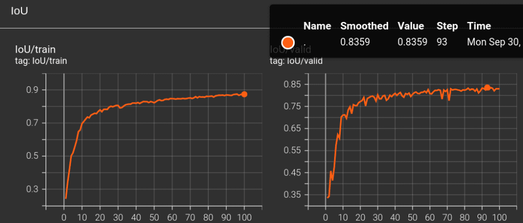
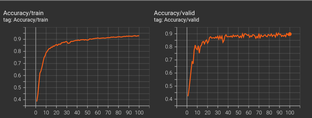
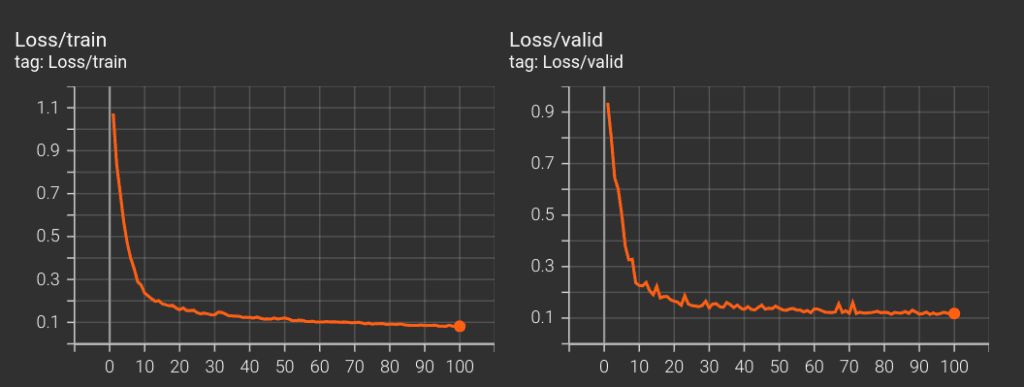
Here is a table listing obtained metrics for all of the experiments carried out for this article.
| Training Config Hyperparams | Loss Function | Model Config | Val IoU |
| init_lr = 1e-3, epochs=120, Multi Step Lr with gamma = 0.1 @ [60,90] | Dice+Focal | No BatchNorm | 80.3 |
| init_lr = 1e-3, epochs=100, Cosine Annealing | Dice+Focal | No BatchNorm | 80.5 |
| init_lr = 1e-3, epochs = 100 | Dice+Focal | BatchNorm | 83.59 |
| init_lr = 1e-4, epochs = 100 | Dice + Focal + Tversky | No BatchNorm | 73.1 |
| init_lr = 1e-3, epochs = 80, Cosine Linear Warmup | Dice+Focal | BatchNorm, Dropout3D | 82.20 |
To interpret the features that contribute the most for model prediction, explainable AI approaches like GradCAM is much helpful. Bookmark our article on GradCAM discussing feature map activation for tumor classification on Brain MRI Scan Data.
Load the best 3D U-Net model weights
Let’s perform inference by loading the best model checkpoint.
DEVICE, GPU_AVAILABLE = get_default_device()
trained_model = UNet3D(in_channels = 3, out_channels = 4)
trained_model.load_state_dict(torch.load("model_checkpoint/3D_UNet_Brats2023/version_0/ckpt.tar", map_location = "cpu")['model'])
trained_model.to(DEVICE)
trained_model.eval()
@torch.inference_mode()
def inference(model, loader, device="cpu", num_batches_to_process=8):
    for idx, (batch_img, batch_mask) in enumerate(loader):

        # Move batch images to the device (CPU or GPU)
        batch_img = batch_img.to(device).float()
        # Get the predictions from the model
        pred_all = model(batch_img)

        # Move the predictions to CPU and apply argmax to get predicted classes
        pred_all = pred_all.cpu().argmax(dim=1).numpy()
        # Optionally break after processing a fixed number of batches
        if idx == num_batches_to_process:
            break

        # Visualize images and predictions
        for i in range(0, len(batch_img)):
            fig, ax = plt.subplots(1, 5, figsize=(20, 8))
            middle_slice = batch_img.shape[2] // 2  # Along Depth
            # Visualize different modalities (e.g., T1ce, FLAIR, T2)
            ax[0].imshow(batch_img[i, 0, middle_slice, :, :].cpu().numpy(), cmap="gray")
            ax[1].imshow(batch_img[i, 1, middle_slice, :, :].cpu().numpy(), cmap="gray")
            ax[2].imshow(batch_img[i, 2, middle_slice, :, :].cpu().numpy(), cmap="gray")

            # Get the ground truth mask as class indices using argmax (combine all classes)
            gt_combined = (
                batch_mask[i, :, middle_slice, :, :].argmax(dim=0).cpu().numpy()
            )

            # Visualize the ground truth mask
            ax[3].imshow(gt_combined, cmap="viridis")
            ax[3].set_title("Ground Truth (All Classes)")
            # Visualize the predicted mask
            ax[4].imshow(pred_all[i, middle_slice, :, :], cmap="viridis")
            ax[4].set_title("Predicted Mask")

            # Set titles for the image subplot
            ax[0].set_title("T1ce")
            ax[1].set_title("FLAIR")
            ax[2].set_title("T2")

            # Turn off axis for all subplots
            for a in ax:
                a.axis("off")
            # Show the plot
            plt.show()


# Run inference
inference(model, val_loader, device="cuda", num_batches_to_process=12)
Inference Results from 3D U-Net
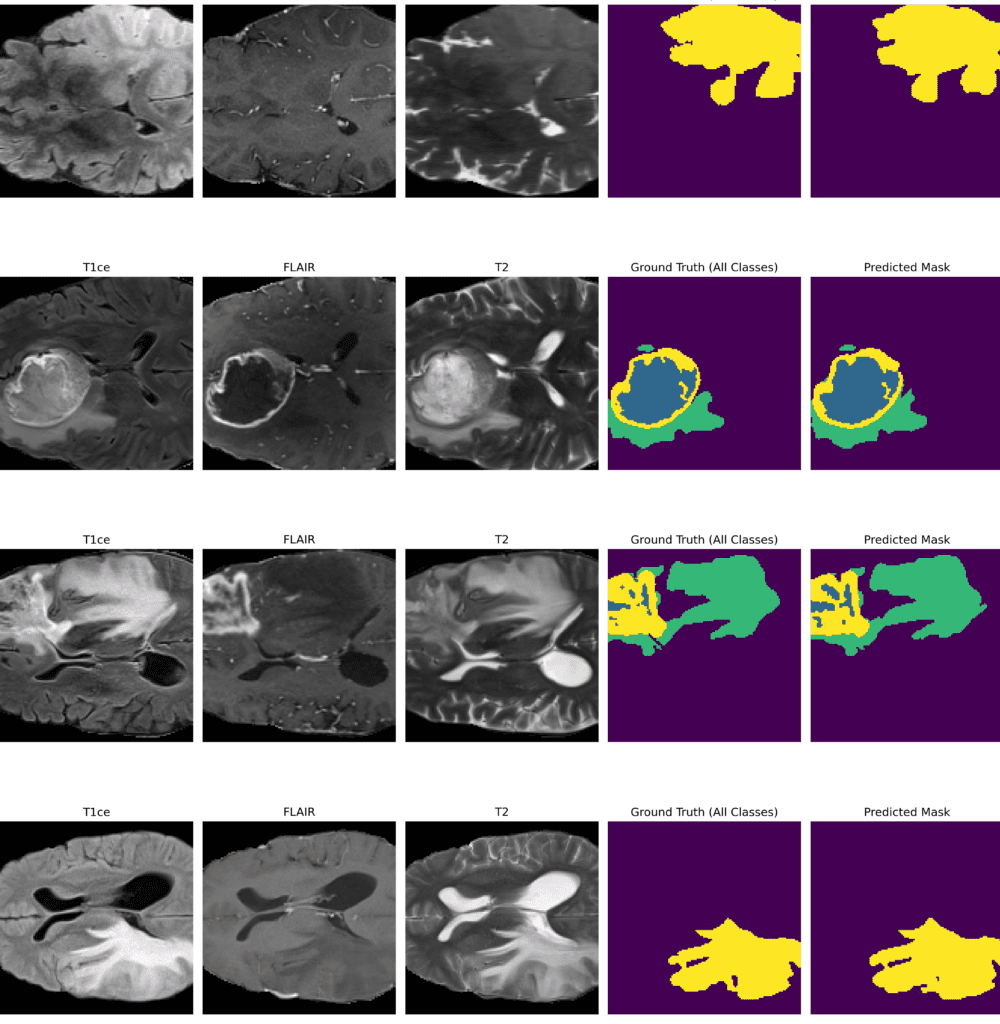
Feel free to pause the video to assess the prediction results.
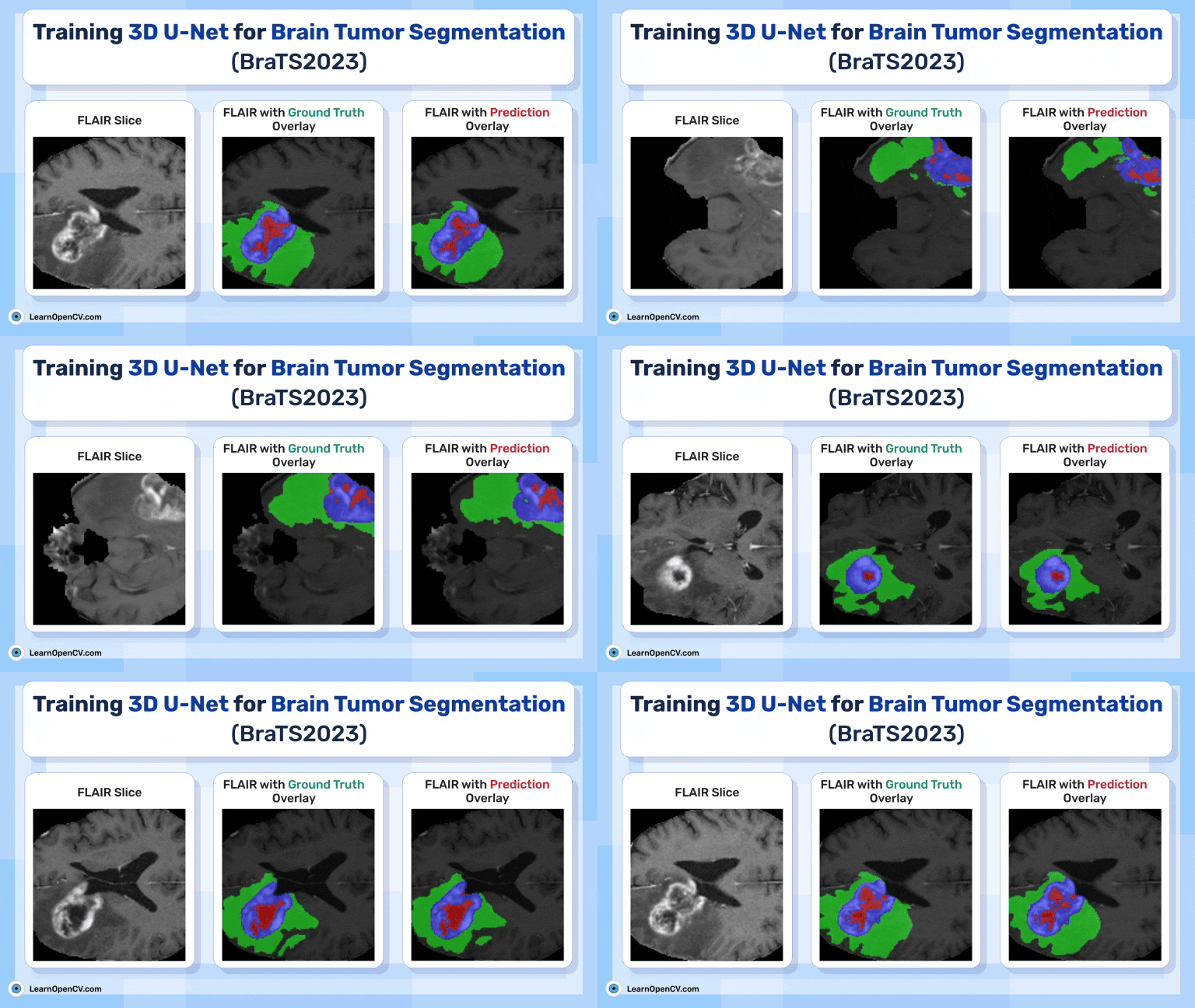
Visualize 3D Predictions as Slices using Trained 3D U-Net
Failure Cases of our trained 3D U-Net model – Not good Predictions
Key takeaways from this article
- Versatility of 3D U-Net: The above set of results demonstrates the effectiveness of our trained 3D U-Net model showcasing its excellence at predicting tumor regions. We achieved a best IoU of 83.59 with BatchNorm layers within the model which helped to stabilize the learning curves. While the results are decent, there is still a room for potential improvement by playing with different training setups and model configuration which is subjected to further experimentation.
- Data Preprocessing: In datasets like these, where the actual ROI are relatively small compared to the entire brain volume, data centric approaches are essential. We cropped the ROI and trained further, this is an effective strategy to speed up training without compromising on the metrics.
- Importance of Loss Function in Medical Segmentation: During inference, in some instances, we observed false positives which are crucial to be addressed especially in medical tasks. In these kinds of scenarios where precision is paramount, choosing the right loss function or combining multiple losses with appropriate parameters such as gamma, alpha and class weights are important which can improve the 3D U-Net’s accuracy thereby minimizing misclassifications.
Conclusion
Extending the well known 2D U-Net to 3D U-Net definitely helped us to handle 3D volumes. While this guide is focussed on BraTS dataset the same approach can be applied to any type of 3D Medical Segmentation dataset, of course with prior data specific preprocessing steps. With use of 3D visualization tools like 3D slicer or celluloid library you can infer better visualization of the segmentation results.
Recent advancements in Zero Shot Segmentation using Segment Anything SAM2 for 3D Medical images such as MedLSAM shows promising results.
If you have got better IoU than our reported metrics, we encourage you to share your insights outlining the choice of training and model configurations that you have employed. We would love to hear them in the comments.
References
- 3D U-Net Paper: https://arxiv.org/abs/1606.06650
- BraTS2023 – Glioma Paper: https://arxiv.org/pdf/2305.19369
- BraTS2023-GLI Winners Approach: https://arxiv.org/pdf/2402.17317v1
- Segmentation Models PyTorch 3D Repository.
- MedSAM: https://github.com/bowang-lab/MedSAM
- MONAI Github: https://github.com/Project-MONAI/MONAI






100K+ Learners
Join Free OpenCV Bootcamp3 Hours of Learning