YOLOv6 Object Detection – Paper Explanation and Inference

YOLO models have become ubiquitous in the world of deep learning, computer vision, and object detection. If you are working on object detection, then there is a high chance that you have used one of the many YOLO models at some point.

In this blog post, we will explore the latest and perhaps the best YOLO model to date, that is, YOLOv6.

YOLOV6 is perhaps the BEST and most improved version of the YOLO models. It has delivered highly impressive results and excelled in terms of detection accuracy and inference speed.

The initial codebase of YOLOv6 was released in June 2022. The first paper, along with the updated versions of the model (v2) was published in September. YOLOv6 is considered the most accurate of all object detectors. This is evident from the fact that the YOLOv6 Nano model has achieved an mAP of 35.6% on the COCO dataset. Also, it runs at more than 1200 FPS on an NVIDIA Tesla T4 GPU with a batch size of 32. To achieve such results, the authors use reparameterized backbones, model quantization, and different augmentations, among many other techniques. We will discuss all these in this blog post.

Through the course of this article, we will not only take a detailed look at the above but will also go through a YOLOv6 tutorial to run inference on videos. We will also compare it with other YOLO versions to uncover the outstanding results and improvements we get with YOLOv6.

• History of YOLO Object Detectors
• What is YOLOv6?
• How Does YOLOv6 Work?
• What’s New in YOLOv6?
• YOLOv6 Model Architecture
• Loss Functions in YOLOv6
• YOLOv6 Improvements for Industrial Applications
• Performance Comparison of YOLOv6 with other YOLO Models
• What Makes YOLOv6 Stand Out?
• How to Use YOLOv6?
• YOLOv6 vs YOLOv5
• Conclusion

YOLO Master Post –  Every Model Explained

Unlock the full story behind all the YOLO models’ evolutionary journey: Dive into our extensive pillar post, where we unravel the evolution from YOLOv1 to YOLO-NAS. This essential guide is packed with insights, comparisons, and a deeper understanding that you won’t find anywhere else.
Don’t miss out on this comprehensive resource, Mastering All Yolo Models for a richer, more informed perspective on the YOLO series.

Mastering All YOLO Models from YOLOv1 to YOLO-NAS: Papers Explained (2024)

History of YOLO Object Detectors

By now, the YOLO family of object detectors includes several repositories and code bases. Here are the prominent ones:

• YOLO Darknet (YOLOv1, YOLOv2, and YOLOv3)
• Ultralytics YOLO
• PPYOLO
• YOLOX
• YOLOv7
• And the latest, YOLOv6

The following table shows some of the many YOLO models along with their model configurations and loss functions.

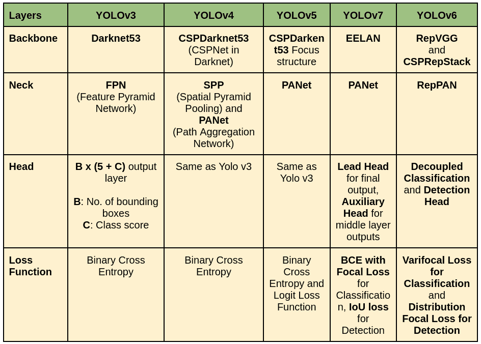
YOLO detectors are constantly evolving, as is evident from new YOLO models being released every few months. With YOLOv6, let’s explore what new and exciting features it brings to the table.

What is YOLOv6?

The YOLOv6 paper was published by researchers at Meituan. It also has a corresponding GitHub repository containing the code, which is being actively maintained and updated. 

The main aim of YOLOv6 is to propagate its use for industrial applications. This demands good performance on a range of hardware and real-world scenarios. Speed and accuracy are paramount for diverse industrial applications. For this reason, YOLOv6 has different models: From the fastest YOLOv6-N (Nano) to the largest and most accurate YOLOv6-L (Large), we have 5 different models to experiment with.

Models in the YOLOv6 Family

The following table gives a comprehensive view of the different models in the YOLOv6 family.

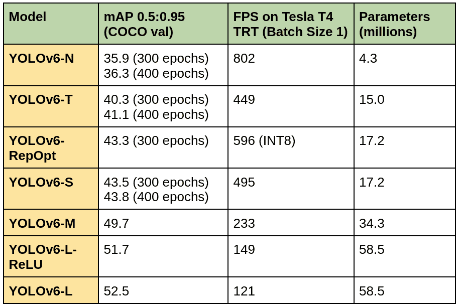
We have YOLOv6-Nano, Tiny, Small, Medium, and Large models in an increasing number of parameters.  

Do you notice the details in the above table? First of all, using the YOLOv6-N model, we get 802 FPS with a batch size of 1 on an NVIDIA T4 GPU with TensorRT. When trained for 300 epochs, we get an mAP of 35.9. But we also have models trained for 400 epochs which give higher mAP. 

The YOLOv6-L model gives an mAP of 52.5 on the COCO validation dataset while still being able to maintain an FPS of 121. 

Also, notice – the RepOpt Small model, the INT8 quantization, and models trained for 400 epochs. As we work through this post, we will gradually uncover how these models were built and what was the motivations behind them.

How Does YOLOv6 Work?

YOLOv6 employs plenty of new approaches to achieve state-of-the-art results. These can be summarized into four points:

• Anchor free: Hence provides better generalizability and costs less time in post-processing.

• The model architecture: YOLOv6 comes with a revised reparameterized backbone and neck.
• Loss functions: YOLOv6 used Varifocal loss (VFL) for classification and Distribution Focal loss (DFL) for detection.
• Industry handy improvements: Longer training epochs, quantization, and knowledge distillation are some techniques that make YOLOv6 models best suited for real-time industrial applications.

What’s New in YOLOv6?

Unlike the previous YOLO architectures, which use anchor-based methods for object detection, YOLOv6 opts for the anchor-free method. 

This makes YOLOv6 51% faster compared to most anchor-based object detectors. This is possible because it has 3 times fewer predefined priors.

YOLOv6 uses the EfficientRep backbone consisting of RepBlock, RepConv, and CSPStackRep blocks. 

Further, YOLOv6 uses VFL and DFL as loss functions for classification and box regression, respectively.

YOLOv6 Model Architecture

Several modern and state-of-the-art practical techniques have been used to make all the YOLOv6 models as fast and accurate as possible.

As with any other YOLO model, the YOLOV6 too has three components. They are the Backbone, the Neck, and the Head of the network, and all have something new to offer. As mentioned earlier, one of the biggest aspects of YOLOv6 is that it is anchor free and uses a reparameterized backbone!

The following image is a complete display of the YOLOv6 object detection model architecture.

As we go along, we will l look at each component of the above image in detail.

The YOLOv6 Backbone Architecture

In any object detection network, the backbone plays a major role in feature extraction. These features are then fed to the neck and head of the network. Hence, the backbone is vital as it is responsible for a major chunk of the computations of the entire network.

Although multi-branch networks like ResNets provide better classification performance, they are slower during inference. Whereas, linear networks like VGG are much faster because of their effective 3×3 convolutions. However, they do not reach as high an accuracy as ResNets or networks with residual connections.

For this reason, the YOLOv6 models use reparameterized backbones. In reparameterization, the network structure changes during training and inference 

For instance, YOLOv6 Nano, Tiny, and Small architectures use reparameterized VGG networks.

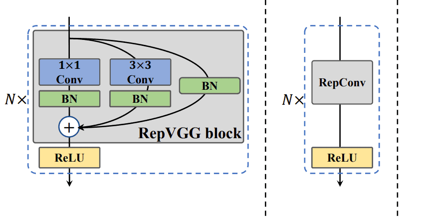
In the above figure, the image on the left shows the reparameterized VGG (RepBlock) block with skip connections. This is used during the training phase of the YOLOv6 architectures. During inference, this changes to simple 3×3 convolutional (RepConv) blocks, as shown in the right image. 

For the Medium and Large models, the YOLOv6 architecture uses reparameterized versions of the CSP backbone. We call it the CSPStackRep.

The entire backbone of the YOLOv6 architecture is called EfficientRep.

The YOLOv6 Neck Architecture

In most object detection models, the neck aggregates the multi-scale feature maps using PAN (Path Aggregation Networks). This is not different in YOLOv6 and similar to what happens in YOLOv4 and YOLOv5.

The PAN in YOLOv6 concatenates features from various reparameterized blocks. For this reason, it is called reparameterized PAN or Rep-PAN for short.

The YOLOv6 Detection Head

Unlike YOLOv4 and YOLOv5, the YOLOv6 architecture used the Efficient Decoupled Head.

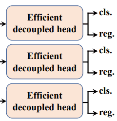
This means that the classification and detection branches do not share the parameters and branch out from the backbone separately. This further reduces computations and provides higher accuracy as well.

Loss Functions in YOLOv6

The YOLOv6 object detection model requires two loss functions. 

• VFL (Varifocal Loss) as classification loss.
• DFL (Distribution Focal Loss) along with SIoU or GIoU as box regression loss

One is for classification and the other is for localization. We can call them classification loss and box regression loss.

Varifocal Loss for Classification

VFL originates from focal loss. This means it already takes care of hard and easy examples during training and weighs them differently.

In addition, VFL also treats the positive and negative examples at different degrees of importance. This helps in balancing the learning signals from both samples.

Distribution Focal Loss for Box Regression

YOLOv6 Medium and Large models use DFL for box regression loss. DFL treats the continuous distribution of box locations as a discretized probability distribution. 

It is especially helpful in detection when the boundaries of the ground truth are blurred. Using DFLv2 was also experimented with, which introduced a lightweight sub-network. But this also meant extra computations, and no improvements over DFL were observed. So, they stuck to DFL as the localization loss function.

YOLOv6 Improvements for Industrial Applications

YOLOv6 is focused on industrial applications, and there are many improvements in this regard.

Longer Training

Few YOLOv6 models were trained for 400 epochs instead of the general 300 epochs. This led to a better convergence

Self-Distillation

YOLOv6 uses knowledge distillation to further improve the accuracy of the models. This is possible without involving a huge computation cost as well.
In knowledge distillation, a teacher model is used to train a student model. The predictions of the teacher model act as soft labels along with the ground truth to train the student model. Essentially, we train a smaller (compared to the teacher) and simpler model and use it to replicate the performance of the teacher model.

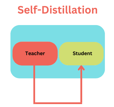
The teacher model can be pre-trained or non-pre-trained, depending on the type of knowledge distillation. Moreover, the teacher model can be a larger model or the same model as well.

As YOLOv6 uses self-distillation for training, the student model acts as the teacher model. In this case, however, the teacher model is pre-trained. 

For training YOLOv6, the optimization process minimizes the KL-divergence between the predictions of the teacher and the student.  

Performance Comparison of YOLOv6 with other YOLO Models

Let’s take a closer look at the training experiments, implementation details, and the comparison of results for the COCO benchmark.

Training Implementation Details

The following table shows the hyperparameters, and hardware details for training the YOLOv6 model.

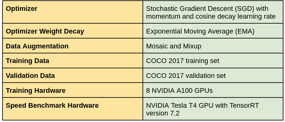
COCO Benchmark and Comparison

The focus was to make YOLOv6 industrial applications ready rather than on the number of parameters involved. This resulted in YOLOV6 having more parameters than its counterparts in the previous versions. But will be more accurate and faster because of the focus on the improvements mentioned earlier.

Now, let’s check out the benchmark comparison of YOLOv6 with previous state-of-the-art YOLO versions:

• YOLOv6 vs YOLOv5
• YOLOv6 vs YOLOv7
• YOLOv6 vs YOLOX
• YOLOv6 vs PP-YOLOE

The following figure shows the comparison of mAP and latency between YOLOv6 and other models.

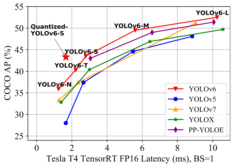
One important observation that can be gleaned from the above figure is that the Quantized YOLOv6-S model is faster and has higher mAP compared to its counterparts in other YOLO versions.

In terms of mAP, all the YOLOv6 models seem to be performing better than the other YOLO versions.

Our observation is strengthened by looking at the following figure, which draws a comparison between the mAP and FPS of various YOLO versions.

Again, the YOLOv6 models stand out to be the most accurate while maintaining at least the same FPS, if not more.

Let’s now look at the quantitative results of COCO 2017 validation set benchmarks.

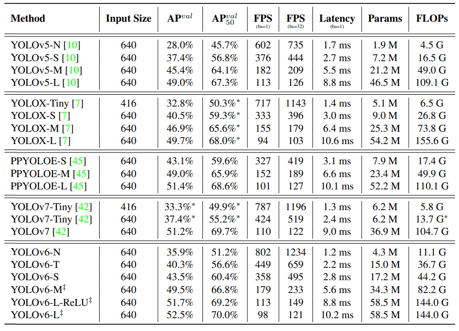
It is as clear as glass that the YOLOv6 models are performing better than the other YOLO models. It is even more astonishing that the YOLOv6-L-ReLU model with 58.5 million parameters is surpassing PPYOLOE-L and YOLOX-L models in both speed and accuracy. And it is on par with YOLOv5-L in terms of FPS but has 1.7% higher AP (at 0.50:095 IoU).

Not only that, but on closer look, you may find that almost all of the YOLOv6 models have higher FPS with batch size 32. This is impressive because the YOLOv6 models seem to have more parameters compared to YOLOv5, YOLOX, YOLOv7, and PPYOLO-E models.

What Makes YOLOv6 Stand Out?

The developers of YOLOv6 carried out several ablation studies to figure out the most impactful of changes.

The ablation studies include:

• Network architecture
• Label assignment strategies
• Loss functions
• Industry-handy improvements
• Quantization strategies

Network Architecture

The authors carried out several ablation studies on the YOLOv6 backbones and necks. These include the RepBlock, CSPStackRep block, and combinations of activation functions and convolutional layers.

The following figures show the tabular results from the YOLOv6 paper.

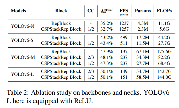
From the above results, it was decided to favor RepBlock for YOLOv6-Tiny, Small, and Nano. And for the Medium and Large models, they went with the CSPStackRep backbones.

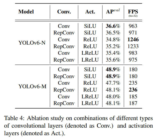
The SiLU activation functions provide the best mAP, but ReLU is faster. For this reason, the official codebase provides a faster ReLU version of the YOLOv6-Large model.

Label Assignment Strategies

Initial experiments show that SimOTA and TAL (Task Aligned Assignment) are the best label assignment strategies for anchor-free object detection models.

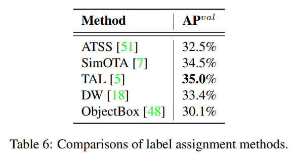
SimOTA, although successful and even used in YOLOX, is slower. Moreover, TAL provides 0.5% compared to SimOTA. Finally, all the YOLOv6 models use the TAL strategy for label assignment.

Loss Functions

YOLOv6 uses VFL as the classification loss function and DFL as the box regression loss function.

The above two were decided through ablation studies.

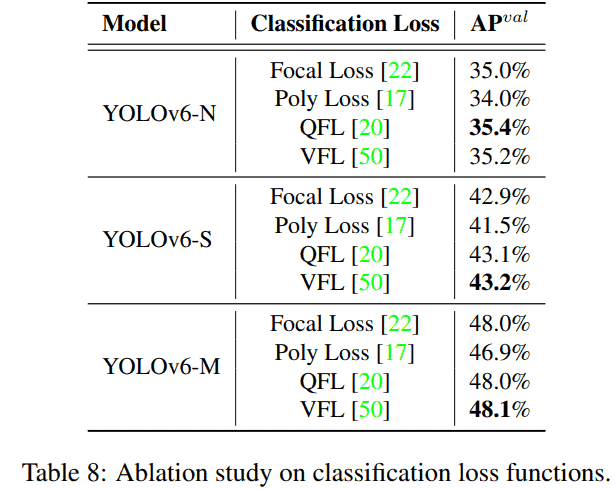
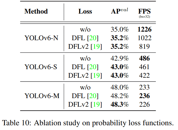
One major change in YOLOv6 is that it doesn’t have an objectness head and, therefore, does not use an objectness loss.

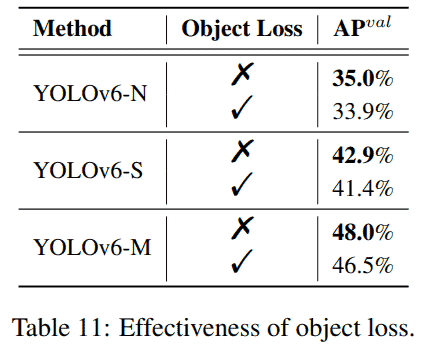
Experiments show that Including the object loss decreases the mAP in YOLOv6-Nano, Small, and Medium models. Also, it does not affect the Large models in a concerning manner. So, they decided not to use the object head in YOLOv6.

Quantization Strategies

The quantization strategies include two experiments:

• Post-Training Quantization (PTQ)
• Quantization Aware Training (QAT)

Most of the quantization experiments were done with the YOLOv6-Small models. However, directly quantizing the models from FP32 to INT8 had negative effects on the mAP. While the FP32 model was giving 42.4% mAP, the INT8 model was giving 35.0% mAP.

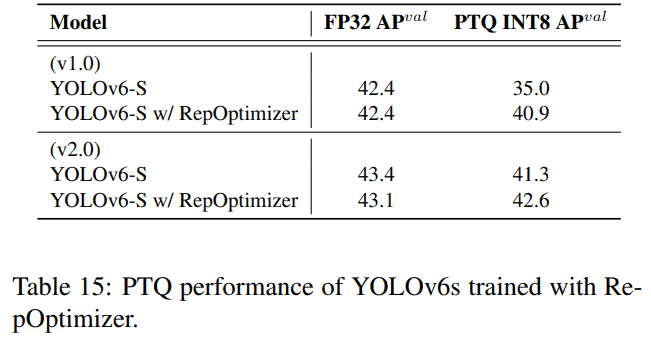
Using Reparameterized Optimizer (RepOptimizer) helped mitigate the issue. As seen from the above figure, using RepOptimizer (with v2.0), the small model only faced a 0.5% drop in mAP.

One other option is QAT (Quantization Aware Training), where we directly train the model with INT8 quantization. With the latest version of the models (v2.0), the authors were able to train the YOLOv6-Small model with full QAT and obtain almost identical results as FP32 or FP16 models.

As we can see from the above table, the YOLOv6-S quantized models are the fastest and most accurate models in their category.

Until now, we have extensively covered all the theoretical details of the YOLOv6 models. Let’s make things more interesting by discussing how to use YOLOv6 models for object detection.

How to Use YOLOv6?

In this section, we will carry out the following inference experiments and comparisons. 

• Using the YOLOv6 pre-trained models for object detection on videos.
• YOLOv5 vs YOLOv6 object detection inference.

You can access the Colab tutorial notebook by downloading it below.

Click here to download the source code to this post

Setting Up YOLOv6 On Local System

Before we come to the inference part, let’s understand how to set up YOLOv6 on our local systems. 

It involves three quick and simple steps

1. Clone the YOLOv6 repository
2. Install the requirements to run YOLOv6 locally
3. Download the pre-trained models

Clone the YOLOv6 Repository

To clone the YOLOv6 repository, simply execute the following command in your directory of choice.

git clone https://github.com/meituan/YOLOv6.git

Now, make YOLOv6 as your current working directory.

Install the YOLOv6 Requirements

Install all the requirements needed to use the YOLOv6 scripts.

pip install -r requirements.txt

Download the YOLOv6 Pretrained Models

The YOLOv6 repository contains all the COCO pre-trained models. You may download the models that you wish to run the inference with.

In the following sections, we will go over several object detection examples using the YOLOv6 pre-trained videos. You may use similar commands and choose the video and model of your choice to run the inference yourself.
If you download the pre-trained weights into the weights folder, the directory structure will look like this:

├── assets
│   ├── banner-YOLO.png
│    ...
│   └── yoloxs.jpg
├── configs
│   ├── experiment
│    ...
│   └── yolov6t.py
├── data
│   ├── images
│   ├── coco.yaml
│   ├── dataset.yaml
│   └── voc.yaml
├── deploy
│   ├── ONNX
│   ├── OpenVINO
│   └── TensorRT
├── docs
│   ├── Test_speed.md
│    ...
│   └── tutorial_voc.ipynb
├── runs
│   ├── inference
│   └── val
├── tools
│   ├── partial_quantization
│    ...
│   ├── infer.py
│   └── train.py
├── weights
│   ├── yolov6l.pt
│   ├── yolov6l_relu.pt
│   ├── yolov6m.pt
│   ├── yolov6m_v2_scale.pt
│   ├── yolov6n.pt
│   ├── yolov6s.pt
│   ├── yolov6s_v2_reopt.pt
│   ├── yolov6s_v2_scale.pt
│   └── yolov6t.pt
├── yolov6
│   ├── assigners
│    ...
│   └── __init__.py
├── infer_drone_video.sh
├── inference.ipynb
├── infer.sh
├── LICENSE
├── README.md
├── requirements.txt
└── turtorial.ipynb

In the above block, all the weight files are inside the weights directory.

Run YOLOv6 Object Detection on Videos

Let’s now look at the inference results after running the inference on the GPU.

Note: All the experiments shown here were run on a laptop with Intel Core i7 8th generation CPU, 6 GB GTX 1060 GPU, and 16 GB of RAM.

The following command shows how to run inference using the YOLOv6 medium model on GPU on a single video.

python tools/infer.py --source video.mp4 --view-img --weights weights/yolov6m.pt --device 0 --name v6m_gpu

The command line arguments are as follows

• --source: The path to the video file. This can also be an image or path to a directory containing multiple images and videos.
• --view-img: This is a boolean flag indicating that we want to visualize the output on the screen.
• --weights: The path to the weights file.
• --device: The computation device. We can either provide cpu, or one digit from 0 to 3 indicating which GPU to use.
• --name: The name of the output directory.

The following video shows the output.

The YOLOv6 Medium model is running around 44 FPS on a laptop 1060 GPU.

YOLOv6 Inference on CPU and GPU

The following video shows the CPU performance of four of the YOLOv6 models, namely Nano, Small, Medium, and Large.

Setting aside the detection quality of the different models, let’s concentrate on the speed. The YOLOv6-Nano model easily runs in real-time, even on the CPU. The Small model is running at a reasonable speed of around 10 FPS. But the Medium and Large models are too slow for CPU inference.

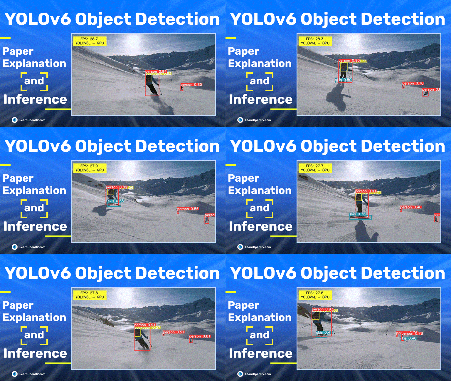
The next video shows the comparison of YOLOv6 models running on the GPU. Notice the differences between the detections from smaller to larger models for the person far away in the frames.

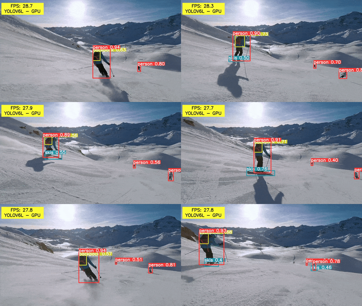
The Small and Nano models are running at more than 160 FPS and 80 FPS, respectively. It is remarkable, considering that we are running this on a laptop GPU. Although the Large model is the slowest (but real-time on the GPU), it is able to detect the person who is farthest in the video. It also detects the backpack in almost all frames, which the other models are missing.

YOLOv6 vs YOLOv5

For comparison purposes, we stack up the YOLOv6 models with their corresponding YOLOv5 versions with similar mAP. We also compare the YOLOv6 models with the YOLOv5x6 (‘x’ representing Nano, Small, Medium, and Large) models. This is because they are the closest in terms of mAP when compared with the YOLOv6 counterparts. 

For example, we may compare YOLO6-Nano with YOLOv5-S and also with YOLOv5-S6.

Let’s take a look at some of the comparison videos.

YOLOv6-Large vs YOLOv5 Models on GPU

Let’s begin with the comparison of two fairly large models. These are the YOLOv5l6 and YOLOv6-L models.

Please note that the YOLOv5l6 model has a slightly higher mAP of 53.7 compared to the 52.5 YOLOv6-L. As YOLOv6 uses more modern techniques, let’s see whether the higher mAP of YOLOv5l6 holds up to its numbers.

There are a few interesting points to note here.

• First of all, both models are running at the same speed. So, everything boils down to the detection quality.
• The YOLOv6-L model is making a few false positive detections. One example is detecting the fuel station as a bus.
• But in the final few frames, the YOLOv6-L model is detecting the cars which appear smaller and are farther away. While the YOLOv5l6 model is not able to do so.

So, it is hard to arrive at a verdict as to which model is better. In the real world, it all depends on the transfer learning performance of the model.

YOLOv6 Nano Model vs YOLOv5 Nano and YOLOv5 Small Models

Here YOLOv6-N has 35.6 mAP, much higher than the mAP of 28.0 of YOLOv5n. For this reason, we also compare the YOLOv5s and YOLOv5n6, which have an mAP of 37.4 and 36.0, respectively. These values are much closer to the mAP of YOLOv6-N.

Right out of the box, we can see that YOLOv5-N is the fastest on CPU, but not by much. The YOLOv6-N is right behind it but more accurate and makes fewer mistakes. YOLOv5-S is the slowest on the CPU, but the most accurate. The YOLOv5-N6 model is as fast as the YOLOv6-N but not as accurate as it is missing out on some of the motorcycle detections in the video.

The following video shows the corresponding comparison but on the GPU.

The detections here will be the same as in the previous video. But the big difference is in the FPS. The YOLOv6-N model is giving good results (almost as good as YOLOv5s) while running at 160 FPS on the GPU.

YOLOv6 Small vs YOLOv5 Small and YOLOv5 Medium Models

Carrying out a similar detection comparison with the YOLOv6-S model on the CPU. For similar reasons as in the above section, we include YOLOv5m (mAP of 45.4) and YOLOv5s6 (mAP of 44.8) in this comparison.

Here, the YOLOv6-S model is running slightly slower compared to the YOLOv5-S model. But the detections are almost identical.

Interestingly, the YOLOv5-S6 model, which is supposed to be more accurate compared to the YOLOv6-S or YOLOv5-S, is giving almost similar results. Maybe even slightly slower compared to the two. One reason could be that the YOLOv5-x6 models have been trained with 1280×1280 resolution images. Whereas, here, we are carrying out inference on 640×640 frames.

The following videos show the same results as above but on the GPU.

Attention newbies:

The following in-depth articles cover different YOLO models, their paper explanations, and the steps to fine-tune them. These have been specially crafted to help you gain a deeper understanding and will go a long way in consolidating your knowledge of the YOLO series. Do read.

• Custom Object Detection Training using YOLOv5
• Pothole Detection using YOLOv4 and Darknet
• YOLOv7 Object Detection
• Fine Tuning YOLOv7
• YOLOX Object Detection

Conclusion

We covered a comprehensive list of topics related to YOLOv6 in this post. To summarise.

• We started with exploring the new components in YOLOv6. This includes the new backbone architecture, loss functions, and training strategies. 
• Then we discussed the experiments and results from the YOLOv6 paper. This gave us a thorough understanding of the performance of YOLOv6 on the COCO dataset.
• We also ran multiple inference experiments using YOLOv6 and observed how it holds up against YOLOv5. We got to observe the FPS and detection quality of several YOLOv6 models with these. 

We would love to hear from you. Please ask your questions in the comment section, and we will answer you right away.

References

• YOLOv6: A Single-Stage Object Detection Framework for Industrial Applications
• YOLOv6 GitHub
• YOLOv6 YouTube preview

Must Read Articles

Here are a few similar blog posts that you may be interested in.

• YOLOv7 Object Detection Paper Explanation and Inference
• Fine Tuning YOLOv7 on Custom Dataset
• YOLOv7 Pose vs MediaPipe in Human Pose Estimation
• YOLOv6 Object Detection – Paper Explanation and Inference
• YOLOX Object Detector Paper Explanation and Custom Training
• Object Detection using YOLOv5 and OpenCV DNN in C++ and Python
• Custom Object Detection Training using YOLOv5
• Pothole Detection using YOLOv4 and Darknet