YOLOv10: The Dual-Head OG of YOLO Series

The classy YOLO series has a new iteration, YOLOv10, a new object detection model. The YOLO series is one of the most used models in the computer vision industry. So, what is YOLOv10? We will explore the answer throughout this article. Whether you are a beginner or an expert, you will have an overview of the entire YOLOv10 architecture, workflow, and real-time inference with some cool results.

To see the experimental results, scroll down to the concluding part of the article or click here to see them immediately.

All the code discussed in this article is free to grab. Just hit the “Download Code” button to get started.

What is YOLOv10?

Three months back, Chien-Yao Wang and his team released YOLOv9, the 9th iteration of the YOLO series, which includes innovative methods such as Programmable Gradient Information (PGI) and Generalized Efficient Layer Aggregation Network (GELAN) to address issues related to information loss and computational efficiency effectively. But just like all other YOLOs, its reliance on the non-maximum suppression (NMS) for post-processing hampers the end-to-end deployment of the model and adversely impacts the inference latency. Additionally, the design of various YOLO components lacks comprehensive inspection, leading to unnecessary computation and reducing the model’s effectiveness.

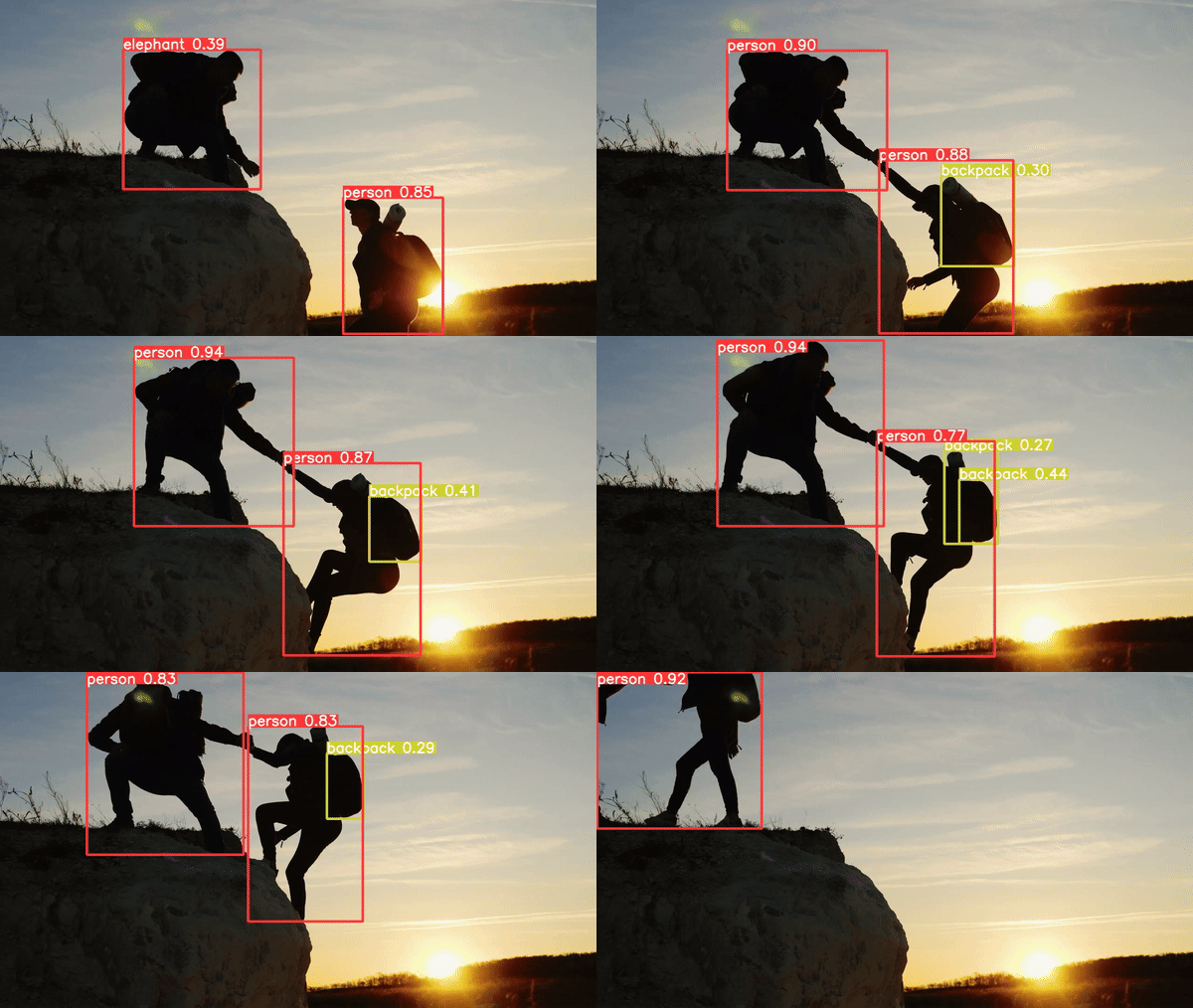
So, like all other YOLOs, Ao Wang, Hui Chen, et al.[1] introduce the latest version of YOLO(v10) with some cool new features. So, what’s new is YOLOv10? YOLOv10 comes with two main upgrades over previous YOLOs: a Consistent Dual Assignments for NMS-free Training and an Efficiency-Accuracy Driven Model Design to improve the overall performance. In the next section, let’s dive deep into these components to understand the root workflow of YOLOv10.

YOLO Master Post – Every Model Explained

Unlock the full story behind all the YOLO models’ evolutionary journey: Dive into our extensive pillar post, where we unravel the evolution from YOLOv1 to YOLO-NAS. This essential guide is packed with insights, comparisons, and a deeper understanding that you won’t find anywhere else.
Don’t miss out on this comprehensive resource, Mastering All Yolo Models, for a richer, more informed perspective on the YOLO series.

Mastering All YOLO Models from YOLOv1 to YOLO-NAS: Papers Explained (2024)

Components of YOLOv10

YOLOv10 consists of two main components: 

1. NMS free training and inference
2. Efficiency-Accuracy Driven Model Design

Let’s explore both of them one by one:

Consistent Dual Assignments for NMS-free Training

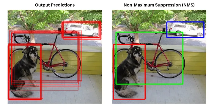
In traditional YOLOs, During training, they usually leverage TAL(Task Alignment Learning)[2] to allocate multiple positive samples for each instance and non-maximum suppression (NMS) to remove redundant bounding boxes for the same object in post-processing. However, NMS can sometimes be a bit of a blunt instrument, potentially discarding useful predictions or failing to remove all duplicates efficiently. Also, it adds more computational cost during the time of training and inference. DETR (DEtection TRansformer)[3]  introduces an elegant way to handle this issue by using the Hungarian algorithm for one-to-one matching during training, thereby eliminating the need for NMS during inference. 

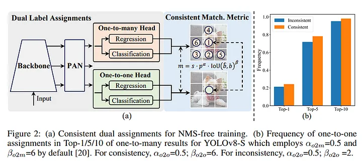
YOLOv10  authors introduced A new architecture to tackle the NMS post-processing with the help of DETR Architecture. It consists of two main components: a dual label assignment using two heads and a consistent matching metric to match both head predictions for a perfect prediction. Now, let’s move to the next section to understand both methods in detail.

Dual Label Assignments

YOLOv10 combines the benefits of one-to-one and one-to-many matching strategies used during the training of object detection models. One-to-one matching assigns only one prediction to each ground truth, simplifying post-processing by eliminating the need for Non-Maximum Suppression (NMS). However, this approach can lead to weaker supervision, resulting in lower accuracy and slower convergence during training. To address this, YOLOv10 gives a dual-label assignment strategy that uses both one-to-many and one-to-one heads during training.

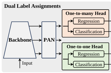
• One-to-Many Head: This head retains the original structure and optimization objectives and benefits the model by dense supervision. During training, it uses one-to-many assignments, which provide rich supervisory signals(features) to the model.

• One-to-One Head: This head uses a one-to-one matching strategy for label assignments, ensuring each ground truth is matched with a single prediction. It operates similarly to the Hungarian matching method but requires less training time. Using one-to-one matching eliminates the need for Non-Maximum Suppression (NMS) during inference, streamlining the prediction process.

In training, both heads are used simultaneously, allowing the backbone and neck of the model to leverage the comprehensive supervision from the one-to-many assignments. This improves the model’s learning and accuracy. The one-to-many head is discarded during inference, and only the one-to-one head is used for making predictions. This approach ensures that the model can be deployed end-to-end without additional computational costs, maintaining high efficiency in real-time object detection tasks. 

Consistent Matching Metric

A consistent matching metric is used to improve YOLOv10’s dual label assignments. This metric ensures that both the one-to-one and one-to-many heads align during their training. The matching metric is defined as

where 𝑝 is the classification score, and 𝑏 are the prediction and instance bounding boxes, and 𝑠 shows if the prediction’s anchor point is within the instance. The parameters 𝛼 and 𝛽 balance the importance of classification and localization tasks. The one-to-many and one-to-one metrics are denoted as and respectively. By using the same metric for both heads, the model ensures the best samples chosen by the one-to-many head are also the best for the one-to-one head.

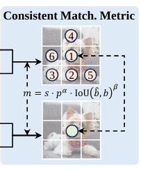
Using the consistent matching metric helps both heads train better together, improving the one-to-one head’s predictions during inference. This metric reduces the supervision gap between the two heads by aligning their training targets. By setting and , both heads pick the same best samples. This alignment has improved performance, as seen by the number of matching pairs between the one-to-one and one-to-many heads after training. This approach leads to better model performance without needing extensive tuning.

Efficiency-Accuracy Driven Model

In addition to post-processing, YOLO models face big challenges in balancing efficiency and accuracy. While various design strategies have been used, there has been a lack of thorough examination of all components in YOLOs. This leads to unnecessary computational load and limits the model’s capabilities. YOLOv10 focuses on balancing efficiency and accuracy in object detection. This involves a series of optimizations in both the model architecture and training processes to maximize performance while minimizing computational costs. Let’s explore both.

Efficiency-driven Model Design

To achieve higher efficiency, YOLOv10 introduces several innovations that reduce computational overhead without sacrificing performance: A lightweight classification head, spatial channel downsampling, and rank-guided block design. Let’s understand each of the components one by one.

Lightweight Classification Head

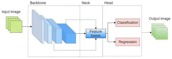
In traditional YOLO models, the classification and regression heads share the same architecture, resulting in high computational costs, particularly for the classification head.

• Classification Head – identifies the class of each detected object, such as ‘person’ or ‘car.’ It also estimates the probability for each class, ensuring the sum of probabilities is one.

• Regression Head – predicts the bounding box coordinates for detected objects, including the center coordinates, width, and height. It also provides a confidence score for each prediction to help filter out low-confidence results.

By analyzing the impact of errors, researchers found that the regression head is more critical for performance. Thus, YOLOv10 adopts a lightweight classification head using two depthwise separable convolutions followed by a 1×1 convolution, significantly reducing the overhead.

Spatial-Channel Decoupled Downsampling

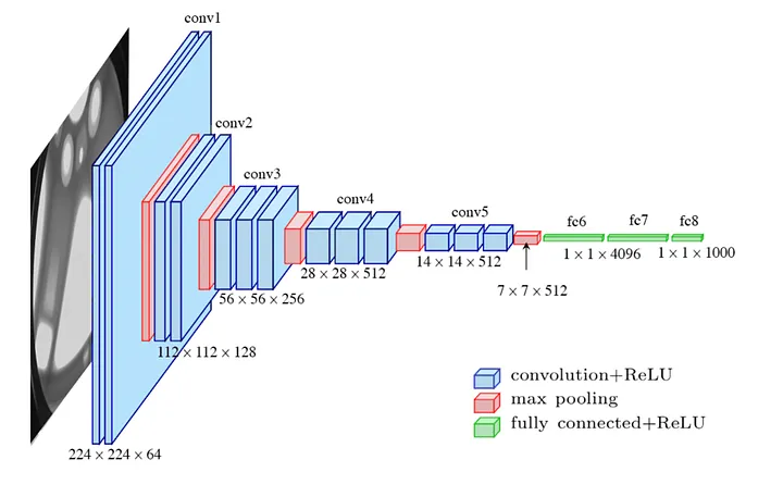
Typical YOLO models use 3×3 convolutions with a stride of 2 for both spatial downsampling(from H × W to H/2 × W/2 ) and channel transformation(from C to 2C), which is computationally expensive. YOLOv10 decouples these operations for greater efficiency. First, a pointwise convolution adjusts the channel dimensions, followed by a depthwise convolution to reduce the spatial dimensions.

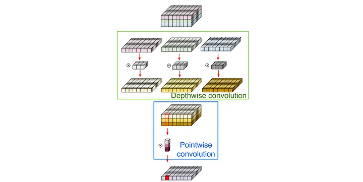
In short, YOLOv10 uses pointwise convolution (1×1 filter) to increase the number of channels and depthwise convolution to reduce the spatial dimensions rather than doing both simultaneously in a single convolution layer. This decoupling reduces computational costs while retaining more information during downsampling. Specifically, the computational cost decreases from to , and the param counts are reduced from to . This approach maximizes information retention and leads to high performance with reduced latency.

Rank-Guided Block Design

YOLOs often use the same block structure across all stages, which can be inefficient and cause bottlenecks. Besides YOLOv9 PGI and GELAN, YOLOv10  introduces a rank-guided block design to address redundancy. It calculates the intrinsic rank of each stage(the last convolution in the last basic block in each stage), identifies redundant stages, and replaces their basic blocks with a compact inverted block (CIB) structure. 

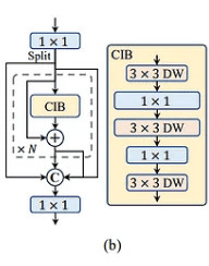
CIB uses depthwise convolutions for spatial mixing and pointwise convolutions for channel mixing. It can be an efficient basic building block, like an embedded part in the ELAN structure(and in the GELAN of YOLOv9). This adaptive strategy first sorts all stages on their intrinsic ranks in ascending order. Then, it replaces the basic blocks(with lower rank) with the more efficient CIB block. The stages are sorted by rank, and these replacements are progressively made to improve performance.

Accuracy-Driven Model Design

To boost accuracy, YOLOv10 comes with two innovative approaches: large-kernel convolution in CIB and partial self-attention. Let’s explore both in the next section.

Large-Kernel Convolution

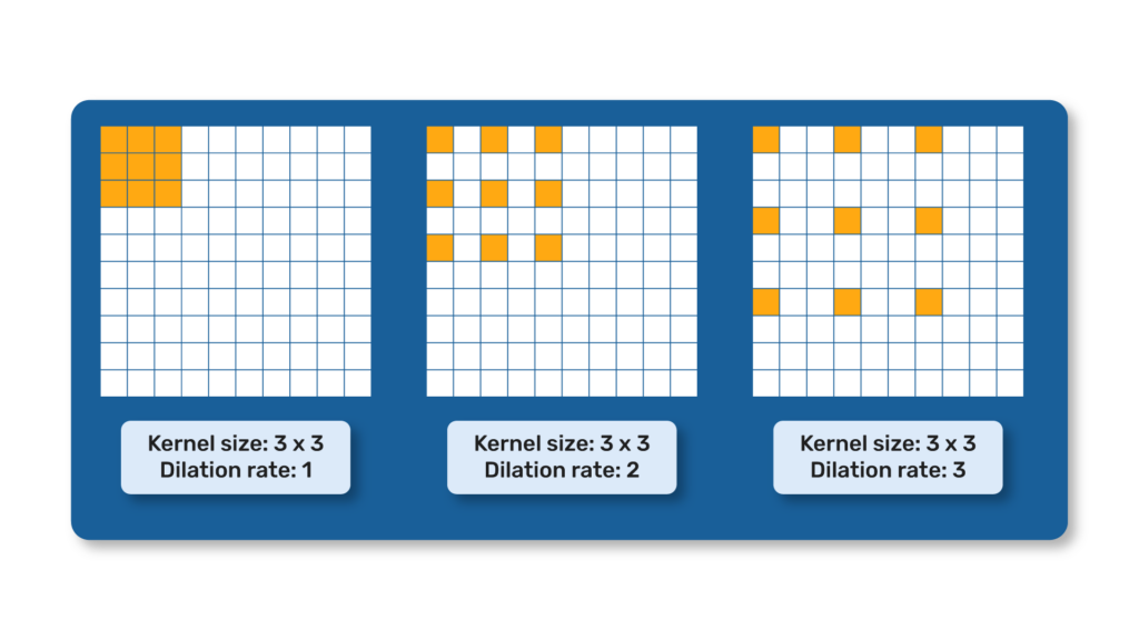
Large-kernel depthwise convolutions are used to enlarge the convolution area size, improving the model’s ability to detect detailed features. YOLOv10 uses these large-kernel convolutions in CIB within deeper stages of the model, specifically increasing the kernel size of the second 3×3 depthwise convolution to 7×7. Additionally, structural reparameterization techniques add another 3×3 depthwise convolution branch to alleviate optimization issues without adding inference overhead. This method improves detection performance, especially for small objects, while keeping the computational load manageable.

Partial Self-Attention (PSA)

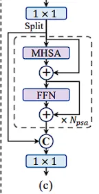
Self-attention[4], while powerful, is computationally intensive. YOLOv10 introduces an efficient partial self-attention (PSA) module to incorporate global representation learning with reduced computational costs. Features are split into two parts after a 1×1 convolution; only one part is processed into the N_PSA blocks comprised of a multi-head self-attention (MHSA) and feed-forward network (FFN). The parts are then concatenated and fused by another 1×1 convolution. PSA is applied only in later stages with lower resolution, avoiding excessive overhead from the quadratic complexity of self-attention. This approach enhances the model’s overall capability and performance with minimal computational cost.

Architecture Overview

The researchers of YOLOv10 hasnt provided the complete architecture diagram as of now. But we can have an architecture overview by understanding the codebase. Let’s explore:

# Parameters
nc: 80 # number of classes
scales: # model compound scaling constants, i.e. 'model=yolov8n.yaml' will call yolov8.yaml with scale 'n'
  # [depth, width, max_channels]
  b: [0.67, 1.00, 512] 

# YOLOv8.0n backbone
backbone:
  # [from, repeats, module, args]
  - [-1, 1, Conv, [64, 3, 2]] # 0-P1/2
  - [-1, 1, Conv, [128, 3, 2]] # 1-P2/4
  - [-1, 3, C2f, [128, True]]
  - [-1, 1, Conv, [256, 3, 2]] # 3-P3/8
  - [-1, 6, C2f, [256, True]]
  - [-1, 1, SCDown, [512, 3, 2]] # 5-P4/16
  - [-1, 6, C2f, [512, True]]
  - [-1, 1, SCDown, [1024, 3, 2]] # 7-P5/32
  - [-1, 3, C2fCIB, [1024, True]]
  - [-1, 1, SPPF, [1024, 5]] # 9
  - [-1, 1, PSA, [1024]] # 10

# YOLOv8.0n head
head:
  - [-1, 1, nn.Upsample, [None, 2, "nearest"]]
  - [[-1, 6], 1, Concat, [1]] # cat backbone P4
  - [-1, 3, C2fCIB, [512, True]] # 13

  - [-1, 1, nn.Upsample, [None, 2, "nearest"]]
  - [[-1, 4], 1, Concat, [1]] # cat backbone P3
  - [-1, 3, C2f, [256]] # 16 (P3/8-small)

  - [-1, 1, Conv, [256, 3, 2]]
  - [[-1, 13], 1, Concat, [1]] # cat head P4
  - [-1, 3, C2fCIB, [512, True]] # 19 (P4/16-medium)

  - [-1, 1, SCDown, [512, 3, 2]]
  - [[-1, 10], 1, Concat, [1]] # cat head P5
  - [-1, 3, C2fCIB, [1024, True]] # 22 (P5/32-large)

  - [[16, 19, 22], 1, v10Detect, [nc]] # Detect(P3, P4, P5)

Backbone

The backbone extracts features from images. YOLOv10 uses an improved version of CSPNet (Cross Stage Partial Network) to improve the flow of information and use less computing power.

Neck

The neck combines features from different backbone levels and passes them to the head. It effectively mixes features from multiple scales(layers) using PAN (Path Aggregation Network) layers.

One-to-Many Head

During training, this head makes several predictions for each object. This gives the model lots of information(features), helping it learn better.

One-to-One Head

During inference, this head makes a single best prediction for each object. This removes the need for NMS (Non-Maximum Suppression), making the process faster.

YOLOv10 – Range of Models

YOLOv10 comes with six variants of models depending on the size and efficiency –

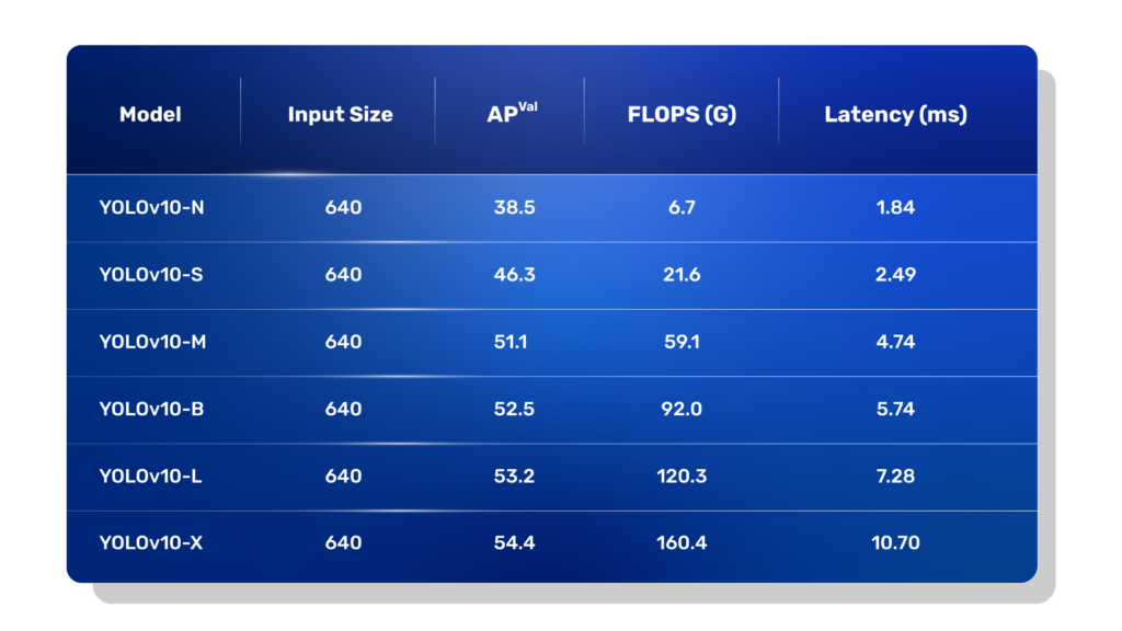
• YOLOv10-N: Nano for small and lightweight tasks.
• YOLOv10-S: Small, upgrade of Nano with some extra accuracy.
• YOLOv10-M: Medium for general-purpose use.
• YOLOv10-B: Balanced with increased width of Medium for improved accuracy.
• YOLOv10-L: Large for higher accuracy with higher computation.
• YOLOv10-X: Extra-large for maximum accuracy and performance.

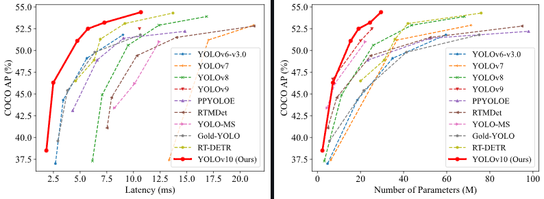
YOLOv10 outperforms previous YOLO versions and other state-of-the-art models in accuracy and efficiency. For example, YOLOv10-S is 1.8x faster than RT-DETR-R18 with similar AP on the COCO dataset, and YOLOv10-B has 46% less latency and 25% fewer parameters than YOLOv9-C with the same performance. YOLOv10-L shows 68% fewer parameters and 32% lower latency than Gold-YOLO-L, with a significant improvement of 1.4% AP. And YOLOv10-X outperforms YOLOv8-X by  0.5 AP with 2.3x fewer parameters.

Click here to download the source code to this post

Inference using YOLOv10 

We’ll use the pre-trained weights from the YOLOv10 GitHub for our inference experiments. To do the inference, you need to clone the YOLOv10 repository by the following command:

! git clone https://github.com/THU-MIG/yolov10.git
! cd yolov10

Then, we need to set up the environment using the following command:

! conda create -n yolov10 python=3.9
! conda activate yolov10
! pip install -r requirements.txt
! pip install -e .

We are using miniconda to create the virtual environment. Within the environment, we installed all the required libraries.

Then, we will run the inference using the following command:

! yolo predict model=yolov10n/s/m/b/l/x.pt source=/path/to/your/video save=True imgsz=384,640

YOLOv10’s codebase is built with Ultrlytics. As described in the Ultralytics documentation, you can use all the available commands for inference. And it’s this easy to do the inference; you are done. The predictions will be saved at the location:

yolov10/runs/detect/predict

Now, all the pre-trained models are available in the pytorch native model, but if you want to export it in the onnx framework, you can do this using the following code:

yolo export model=yolov10n/s/m/b/l/x.pt format=onnx opset=13 simplify

You can add or modify other parameters using the ultralytics documentation. We are done with the code; see the result now:

Cool right! Now, let’s compare some inference results below.

YOLOv8 vs YOLOv9 vs YOLOv10

Now, we will compare the last three iterations of the YOLO series. We will compare the results visually and also compare the benchmarks. I have taken the YOLOv10L(24.4M params), YOLOv9C(25.3M params), and YOLOv8M(25.9M params) for our experiment to maintain inference similarity. We used Nvidia Geforce RTX 3070 Ti Laptop GPU to run the inference and set the imgsz=384,640 for all models. The results are here:

You can see that YOLOv10 and V9 can detect smaller objects(birds here) more efficiently. 

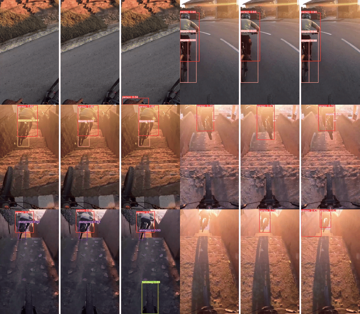
Here, we observed the No. of false predictions are less in YOLOv10 than others, and the conf. score is much better in YOLOv10 as well.

In this case, YOLOv9 performed better than the other two. 

Here, YOLOv10 performs well compared to the other two. Though all three detect the fish as kites, YOLOv10 has the minimum number of false detections.

Here also, the false detection is less in YOLOv10.

In this case, all the models performed well. However, as we worked with the default parameters, YOLOv10 is not able to detect some small objects in the distance, e.g., the person in the subway(in the third video) and the person in the distance in the left-down corner(in the fifth video). To tackle the issue, the authors of YOLOv10 suggest to set a smaller confidence threshold for inference.

Interesting results, right? Click here to get an overview & play with the code. Tune all the parameters according to your use case, and get your hands dirty.

Now let’s see a comparison benchmark of these three models in terms of numbers:

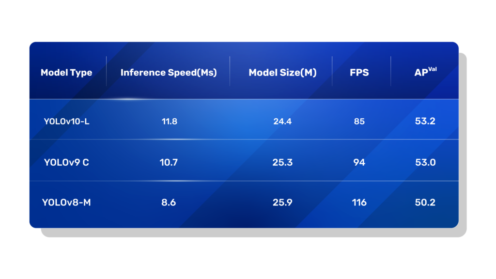
The benchmark results show that each model has its own strengths. YOLOv8 achieved the highest fps for me. Now, let’s move on to more benchmark results, specifically YOLOv10. 

YOLOv10 – Benchmarks

We divided the Benchmark comparison into two separate experiments. First, we will compare the pytorch native and the exported onnx version of the YOLOv10B model. We used Nvidia Geforce RTX 3070 Ti Laptop GPU to run the inference and set the imgsz=384,640 for both models. We used the same video for inference with both models, and here are the results:

YOLOv10B.onnx - Speed: 0.9ms preprocess, 11.5ms inference, 0.3ms postprocess per image at shape (1, 3, 384, 640)
YOLOv10B.pt - Speed: 0.9ms preprocess, 9.9ms inference, 0.6ms postprocess per image at shape (1, 3, 384, 640)

In our case, we got a lower inference time for the pytorch(.pt) model. We got a higher FPS for the pytorch native model(101FPS) than the onnx model(86FPS). 

Next, to elaborate, I used a file directory containing 15 videos as input for both models. And the benchmarks are here:

YOLOv10B.onnx - Speed: 1.3ms preprocess, 12.4ms inference, 0.4ms postprocess per image at shape (1, 3, 384, 640)
YOLOv10B.pt - Speed: 1.2ms preprocess, 10.1ms inference, 0.7ms postprocess per image at shape (1, 3, 384, 640)

In this case, The FPS of the pytorch model(99) is also higher than the onnx version(80).

Now, the 2nd part. Here, we will compare the YOLOv10N, YOLOv10M, YOLOv10B, YOLOv10L, and YOLOv10X models. We take the same video file directory of 15 videos to run the inference in both models. We used Nvidia Geforce RTX 3070 Ti Laptop GPU to run the inference and set the imgsz=384,640 for all models. Here are the inference benchmarks:

YOLOv10N - Speed: 1.1ms preprocess, 4.0ms inference, 0.6ms postprocess per image at shape (1, 3, 384, 640)
YOLOv10M - Speed: 1.1ms preprocess, 7.5ms inference, 0.7ms postprocess per image at shape (1, 3, 384, 640)
YOLOv10B - Speed: 1.1ms preprocess, 9.5ms inference, 0.7ms postprocess per image at shape (1, 3, 384, 640)
YOLOv10L - Speed: 1.2ms preprocess, 11.8ms inference, 0.7ms postprocess per image at shape (1, 3, 384, 640)
YOLOv10X - Speed: 1.2ms preprocess, 14.9ms inference, 0.8ms postprocess per image at shape (1, 3, 384, 640)

As we can observe, all the models took minimal time to perform the inference with a decent FPS. We used all the pre-trained weights provided with YOLOv10 and default parameters to run the inference. Due to that, in the non-exported format, e.g., pytorch, the speed of YOLOv10 is biased because the unnecessary cv2 and cv3 operations in the v10Detect are executed during inference. YOLOv10 authors provided a solution for that; we have to set the export attribute of v10Detect to True before the measurement using the pytorch model. We will explore these suggestions in one of our future articles.

Now that we are done with the benchmarks, let’s look at this article’s key takeaways for a quick recap.

Key Takeaways

Dual Assignments for NMS-free Training

YOLOv10 introduces a dual-head architecture, combining one-to-many and one-to-one label assignments during training. This innovative approach eliminates the need for Non-Maximum Suppression (NMS) during inference, streamlining the prediction process and enhancing efficiency without sacrificing accuracy.

Efficiency-Accuracy Driven Model Design

YOLOv10 employs an Efficiency-Accuracy Driven Model Design, including lightweight classification heads, spatial-channel decoupled downsampling, and rank-guided block design. These optimizations reduce computational overhead and improve performance, ensuring a balance between efficiency and accuracy in object detection tasks.

Performance Improvements Over Other YOLOs

YOLOv10 outperforms previous YOLO versions and other state-of-the-art models in terms of both accuracy and efficiency. It significantly improves latency and parameter counts while maintaining or enhancing detection performance, especially for small objects.

Perfect Benchmarks

Extensive benchmarking reveals that YOLOv10 models exhibit high inference speeds and accuracy across various sizes (Nano to Extra-large) with low latency effectively. YOLOv10 models demonstrate superior performance metrics compared to their predecessors, making them ideal for real-time object detection applications.

Conclusion

YOLOv10 represents a significant leap forward in object detection. It addresses previous limitations in the YOLO series by integrating Consistent Dual Assignments for NMS-free training and an Efficiency-Accuracy Driven Model Design. These advancements result in faster, more accurate detections while reducing computational costs. So, next time you have an object detection task, make sure to use YOLOv10 for quick and precise results.

This article has been added to the Official YOLOv10 GitHub README by the makers of YOLOv10

Reference

[1] Wang, Ao, et al. “YOLOv10: Real-Time End-to-End Object Detection.” arXiv preprint arXiv:2405.14458 (2024).

[2] C. Feng, Y. Zhong, Y. Gao, M. R. Scott and W. Huang, “TOOD: Task-aligned One-stage Object Detection,” 2021 IEEE/CVF International Conference on Computer Vision (ICCV), Montreal, QC, Canada, 2021, pp. 3490-3499, doi: 10.1109/ICCV48922.2021.00349.

[3] Carion, Nicolas, et al. “End-to-end object detection with transformers.” European conference on computer vision. Cham: Springer International Publishing, 2020.
[4] Vaswani, Ashish, et al. “Attention is all you need.” Advances in neural information processing systems 30 (2017).