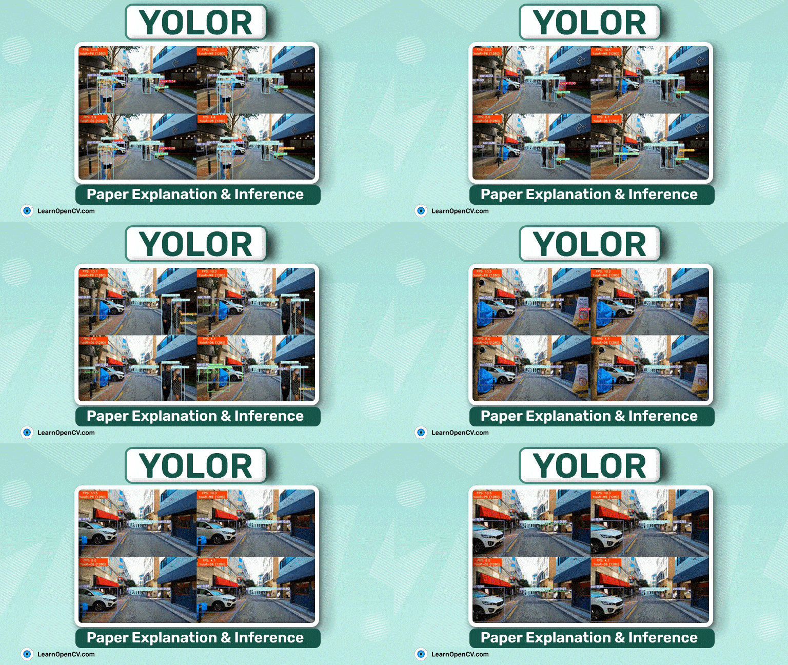
In recent years, we have seen tremendous progress in the YOLO series, now hosting both anchor-free and anchor-based object detection models. Instead of focusing solely on architectural changes, YoloR takes a new route. It takes inspiration from how humans combine implicit knowledge with explicit knowledge to tackle unseen tasks. The proposed techniques significantly improve the performance of the YoloR object detection models, resulting in them being ~88% 🚀 faster and better (🎯 57.3% on the COCO test set) with minimal additional cost.
What will we learn through the course of this article?
- What is YoloR? What’s new!!
- The intuition behind YoloR and how it works.
- Architectural changes and differences among the YoloR models.
- A comparative inference analysis of YoloR models.
- Who Are The Authors Of YoloR?
- Is YoloR Worth Exploring?
- What is YoloR?
- What’s Different in YoloR?
- YoloR – A Unified Network
- YoloR Architecture
- How Is Implicit Knowledge Useful In A Network?
- Formulation of Implicit Knowledge In Unified Networks
- Paper Experiments
- YoloR Object Detection Inference
- Summary
YOLO Master Post – Every Model Explained
Don’t miss out on this comprehensive resource — Mastering All Yolo Models for a richer, more informed perspective on the YOLO series.
Who Are The Authors Of YoloR?
The authors of YoloR are Chien-Yao Wang, I-Hau Yeh, and Hong-Yuan Mark Liao. Along with Alexey Boschovskiy, these four authors have been involved in the development of CSPNet, YoloV4(2020), Scaled-YoloV4 (2020), and YoloV7 (2022). YoloV4 was a critically acclaimed paper to which Scaled-YoloV4 made further improvements. Scaled-YoloV4 was an “architecture improvement paper.” YoloR (2021) is based on Scaled-YoloV4 models and has its own take on improving the results further.
Is YoloR Worth Exploring?
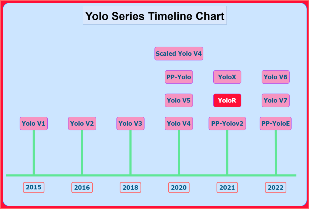
The authors of the YoloR paper take a “roads untraveled” approach for further improvement of the Yolo series. The empirical and comparison results published by the authors show that the new approach has some strong validity. Besides, YoloR-D6 (2021 – 57.3%) performs better than the (best) YoloV7-E6E model (2022 – 56.8%) on the COCO test-dev set.
This is not a diss on the YoloV7. For example, in this validation mAP comparison of YoloV7 with YoloR and other models, you can see the superiority of YoloV7.
They are both excellent papers that use different techniques for improvements and are creditworthy.
New YOLOR (Scaled-YOLOv4-based) is better than new ConvNeXT, SWIN, Detr, YOLOX, PP-YOLOv2, YOLOv5, EfficientDet…https://t.co/YFim1oKXfIhttps://t.co/NgO9wtRzwYhttps://t.co/IelcU2Bmnw
— Alexey Bochkovskiy (@alexeyab84) January 14, 2022
SWIN is so slow that it needs a logarithmic latency scale to fit on the chart… pic.twitter.com/xAgU1gnWiT
As mentioned above, the YOLO series now hosts anchor-less and anchor-based models.
💡 Did you know the first Yolo model released in 2016 was also an anchor-less object detection model?
The whole anchor-less detection mechanism was brought to mainstream attention by two other models. That honor goes to the FCOS object detection model, which approaches the problem in a per-pixel prediction fashion, similar to segmentation. And, CenterNet, which models an object as a single point.
Finally, we arrive at YoloX anchor-less object detection model (2021), released around the same time as YoloR. YoloX was good but not as good as YoloR. YoloX delivered on-par results with other state-of-the-art (SOTA) models.
⚡ You may be surprised to learn that the current SOTA architecture in terms of real-time detection is YoloV6, an anchor-less object detection model.
What Is YoloR?
As we are aware, the Yolo series primarily tackles the problem of object detection. This paper is no different in that aspect. YoloR stands for “You Only Learn One Representation: Unified Network for Multiple Tasks.” the second part of the title states something new and unexplored in other Yolo versions.
The authors of YoloR aimed to create:
“A unified network that can generate a unified representation to serve various tasks simultaneously.”
Their goal is to create a single model capable of learning general representations. Then each sub-network can utilize these representations to create suitable sub-representations for solving a task. A task can be classification, detection, pose estimation, object tracking, etc.
The origins of YoloR lie in the problem faced during the Multi-Task Joint Learning network training. When training a single model that can solve multiple tasks, i.e., joint optimization, each sub-network tends to pull the weights in the direction suitable to itself. This often leads to the poor generation of general features, causing the final overall performance to be worse off than training multiple models individually.
We’ll go deeper to understand the meaning of “unified network” in the following sections.
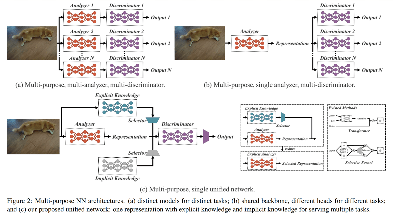
Referring to the above image:
- In Figure 2(a): We have multiple separate networks for each task.
- In Figure 2(b): We have the typical architecture of a multi-task network.
- In Figure 2(c): The proposed unified network (combining explicit and implicit knowledge) architecture that generates one unified representation for serving multiple tasks.
What’s Different In YoloR?

The authors of YoloR (successfully) take on a new direction unexplored by other papers in the Yolo series for model improvements.
Humans rely on their physical senses and past experiences to understand their surrounding environment. Over the years, we have built a massive database of knowledge and experience gained through regular learning (explicit knowledge) or subconsciously (implicit knowledge) stored in our brains. These two types of knowledge, explicit and implicit, in combination, effectively help us function with ease regularly.
The inspiration for YoloR comes from how humans effectively combine the information perceived from the surrounding environment with their past knowledge and experiences to process data previously unseen.
The main focus of this paper is:
“…to create a unified network that can encode and combine implicit and explicit knowledge, just like the brain can learn from normal and subconscious learning.”
In YoloR object detection models, implicit knowledge encoded by the network is used for kernel-space alignment and prediction refinement. When enhanced with implicit knowledge, representations generated by networks can be used to solve the challenges faced with multi-task networks.
For object detection, YoloR relies on predefined anchor boxes similar to Scaled-YoloV4.
YoloR – A Unified Network
In the previous sections, new terms were used, such as “unified network” and “explicit and implicit knowledge.” In this section, I’ll explain these points and what they mean in the context of neural networks.
What Is Meant By Explicit & Implicit Knowledge?
From a psychological perspective, the theory behind the “different types of knowledge” is vast. However, from the paper’s point of view, the following is all you need to know:
- Explicit Knowledge: The knowledge that is easy to articulate, write down, and share with others is known as explicit knowledge. It can be codified and digitized in books, documents, reports, memos, etc.
- Implicit and Tacit knowledge: The knowledge gained from experience are more difficult to express and deeply embedded in the brain. Personal wisdom, insights, intuition, and expertise are context-specific and more difficult to extract and codify. For example, skills learned on a job that is transferable to different positions/jobs, i.e., knowledge acquired from experience. It refers to knowledge learned in a subconscious state.
In reality, implicit knowledge differs from tacit knowledge, but in the YoloR paper, they are considered one.
How Do Humans Understand & Learn New Things?
The YoloR paper begins by asking a loaded question, which is also the source of inspiration for the paper.
Human beings have grown/evolved through centuries by perceiving their surrounding environment and using proactive and reactive measures.
Experience and intuition are integral parts of human knowledge. Without them, it might be difficult to “make sense of” or “react to” a new environment. We function daily at a high level with ease using information about the surrounding environment from our sensory organs and the knowledge/experience/intuition stored in our brains.
When we encounter a new situation or problem, we rely heavily on our past experience and information perceived from the surroundings to understand, interpret and react in the best way possible. Ultimately, we can say we’ve gained more knowledge (new experience) which is now part of our database.
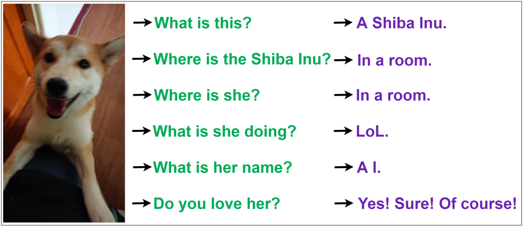
Take the above image as an example. Humans can analyze it from different perspectives with ease. We can easily classify and answer various questions for the same data.
This is not entirely true for neural networks. A CNN trained for classifying “what is this?” will work perfectly well (with some margin of error) on classifying the above image. Still, if we change the task to “where is she?” the model is either not helpful or needs to be retrained or trained in a multi-task setting.
The reason is that the features learned (on one task) and extracted from a trained CNN model are poorly adaptable to other problems. And we only use the network for feature extraction. Still, the implicit knowledge, abundant in a network, is ignored.
The implicit knowledge of the trained model can be thought of as its ability to understand and decide where to look, what, how, and which features to extract and combine to create meaningful feature representations.
Just like humans apply our past experiences to understand and approach a new problem, in this paper, the authors try to encode the implicit knowledge of neural networks so that it can be used for multiple new tasks.
What’s It All To Do With Neural Networks? How Do We Relate Them?
From CNN’s point of view, features extracted from the shallow layers, which constitute edges, corners, curves, etc., are heavily related to the input. The extracted features are often called explicit knowledge, as they are derived directly from the input. In contrast, features obtained from the deeper layers are known as implicit knowledge.
The features extracted by the model become more and more complicated and harder to interpret. The information has been deeply encoded in higher dimensional space, which only the network can understand and use.
“In this paper, we call the knowledge that directly correspond to observation as explicit knowledge. As for the knowledge that is implicit in the model and has nothing to do with observation, we call it as implicit knowledge.”
To understand this, let’s take another example. Suppose you are given a network figure and have to find the number of parameters.
When you first look at the network, you realize you haven’t seen that type of structure before. Yet, you recognize the essential components/layers of the network. First, you’ll extract vital information from the diagram, such as the number of nodes per layer, number of layers, connections, etc. Next, you’ll start calculating the number of parameters per node/layer because you understand the steps to perform and the methodology to use to solve the problem.
Two things:
- We observed and extracted the information from the problem — this is explicit knowledge.
- We used our past knowledge — implicit knowledge; combined it with the current observation to solve the problem.
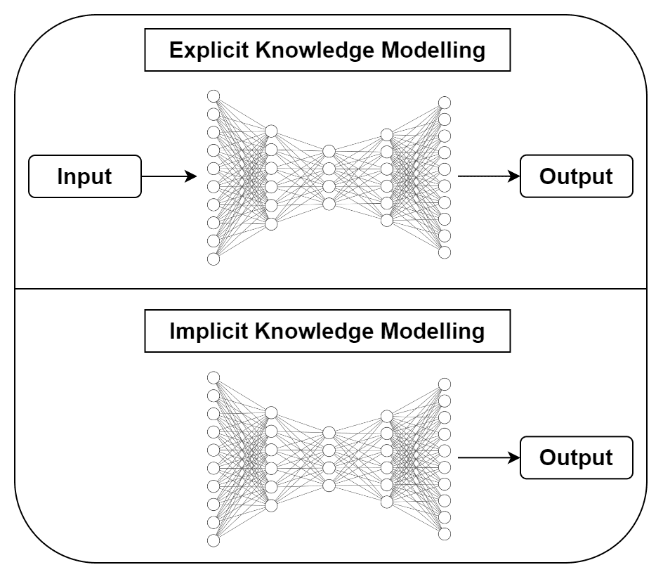
As mentioned in the above example, explicit knowledge relies on the input to generate an output, while implicit knowledge doesn’t.
Hopefully, by this point, you understand the concept of explicit and implicit knowledge, the intuition of the paper, and how it relates to neural networks.
A question arises, “But how does it actually look?”
- The explicit knowledge is being modeled (learned) by a neural network that takes in inputs and produces output. It can be any architecture (YoloV3, EfficientDet, etc.).
- Implicit knowledge – In this paper, the authors have provided three methods we can use to model implicit representations. We will look at this in the next sections, where we’ll go over all three modeling techniques (don’t worry, it’s easier than it feels like) and how to combine them with the explicit knowledge network.
YoloR Architecture
As previously mentioned, the YoloR models are built upon the Scaled Yolov4 architecture. The authors take the Scaled YoloV4-P6 as the base model.
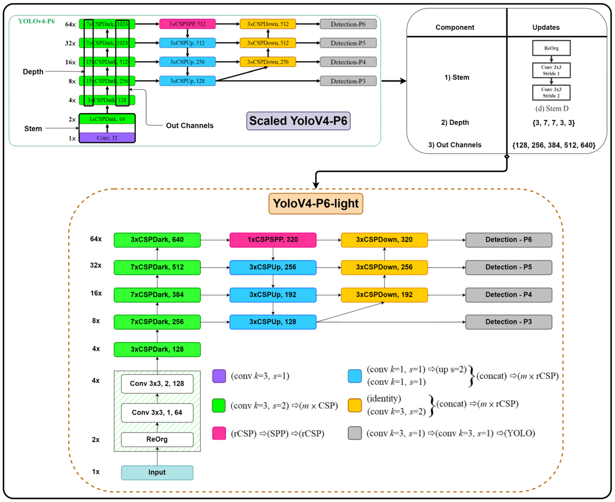
First, a light version: YoloV4-P6-light, is constructed by changing the following:
- The Stem of the network to reduce the input size and the number of parameters.
- A significant reduction to each backbone stage’s Depth and Out Channels. Accordingly, the channels in the neck of the model are also updated.

The YoloR models use the Yolov4-P6-light model as the base architecture. The authors have provided 4 model variants in the paper: P6, W6. E6 and D6.
- YoloR-P6 is created by simply changing the activation function from Mish to SiLU.
- YoloR-W6 uses YoloR-P6 architecture and changes the number of channels used in each backbone stage and, consequently, the neck.
- YoloR-E6 is created by scaling the channels of YoloR-W6 by 1.25 times and changing all downsampling modules from strided Convolution to CSP convolution.
- Finally, the YoloR-D6 is a collective model of all the above changes with increased depth of the backbone stages.

How To Model Implicit Knowledge?
So far, we’ve just talked about modeling the explicit knowledge network. Next, let’s discuss the methods to model implicit knowledge.
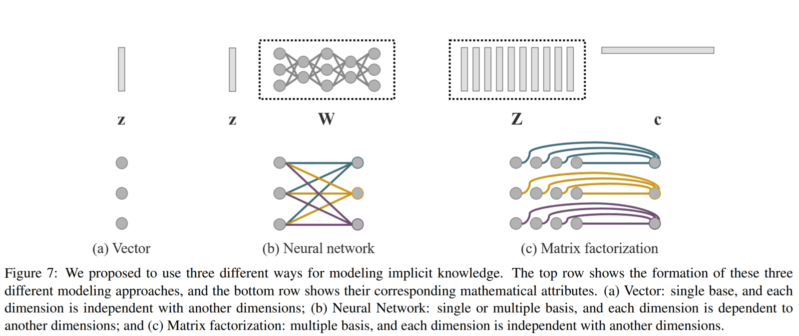
The YoloR paper provides three methods by which we can model implicit knowledge.
- Vector / Matrix / Tensor (z): Using a vector z as the prior of implicit knowledge and directly as implicit representation.
- Neural network (Wz): Use vector z as the prior of implicit knowledge, then use the weight matrix W to perform linear combination or non-linearization, which can be used as an implicit representation.
- Matrix Factorization (ZTc): Use multiple vectors as prior of implicit knowledge, and these implicit prior basis Z and coefficient c will form implicit representation.
All representations mentioned use trainable parameters and are updated alongside the model parameters during backpropagation.
How Is Explicit & Implicit Knowledge Combined?
The authors use three types of operators to combine explicit and implicit knowledge: addition, multiplication, and concatenation.
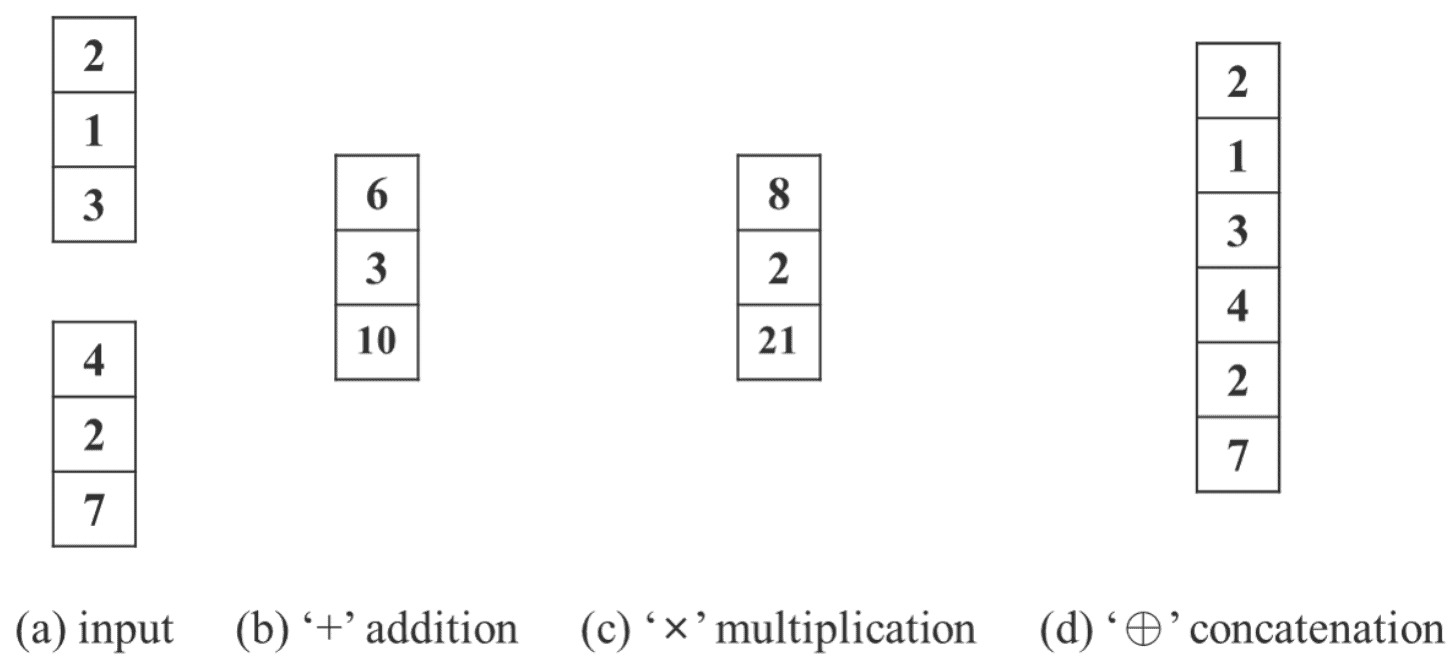
Specifically, in YoloR:
- Implicit knowledge is modeled using the vector/matrix representation.
- For combining with explicit knowledge, addition and multiplication operator are used.
Complete Architecture Of YoloR-P6

In the YoloR models, implicit knowledge has been modeled using trainable vector representations.
Two implicit representations are used:
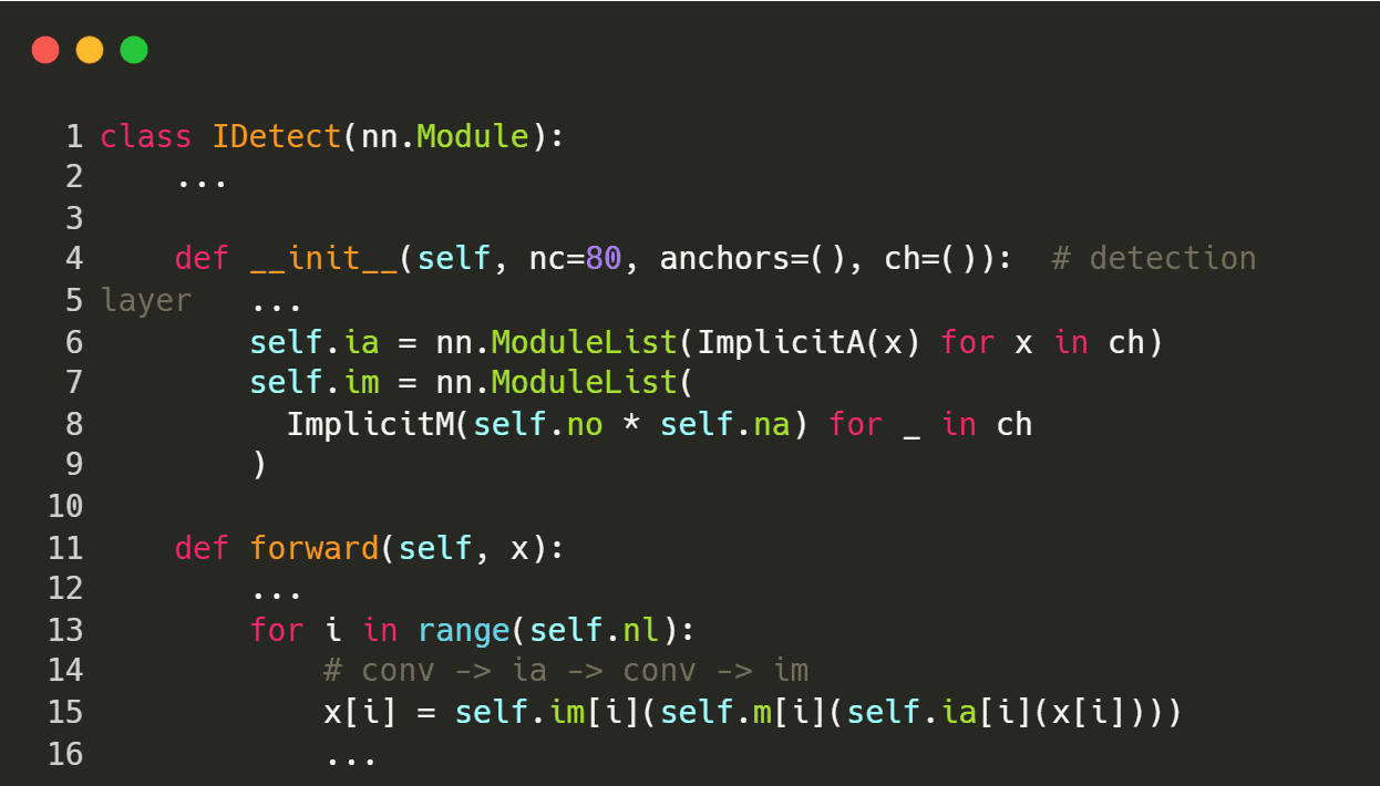
- The first is to help with the kernel space misalignment problem. It is combined with explicit knowledge using the addition operator: ImplicitA.
- The second one is for prediction refinement, combined using the multiplication operator: ImplicitM.
Note: The Conv layer ahead of CSPDown blocks are also present in Scaled YoloV4-P6 and YoloV4-P6-light. It has been added in this diagram to showcase the input and placement of the two implicit representation
Code for initializing Implicit knowledge tensor representation (paper branch)
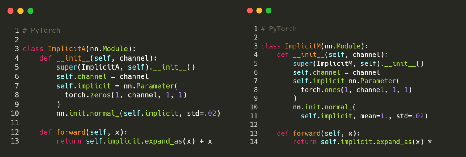
Combining with explicit knowledge
How Is Implicit Knowledge Useful In A Network?
As you may have guessed by now, the crucial part of this research is how we can effectively create an implicit knowledge base in neural networks. In this section, we’ll review some scenarios the authors have mentioned in the paper to understand how implicit knowledge can be applied to various tasks.
Let’s say we have a representation of implicit knowledge for “k” tasks as a set of constant tensors.

Use In Manifold Space Reduction
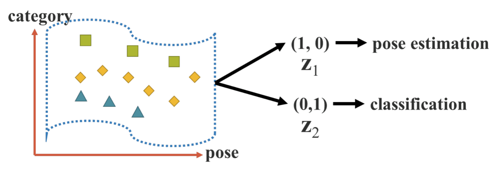
Take the above image as a reference. Let’s assume that the blue-colored wave plane is in a 3D space, and we have projected the points (squares, rhombus, triangles) to 2d (this is a good representation). Let’s say that z1 and z2 from our implicit representation set are for classification and pose estimation tasks with vectors (0, 1) and (1, 0), respectively.
Considering the classification task and points in 2D space, it’s clear that if we could somehow project the points onto the y-axis, we could easily categorize them all. In the above example, we can take the inner product of the projection vector (3D to 2D) and implicit representation z1 to reduce the dimensionality of manifold space and effectively achieve the task.
Use In Kernel Space Alignment
In multi-task and multi-head neural networks, kernel space misalignment is a common problem.
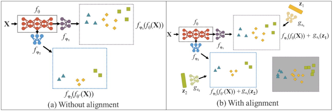
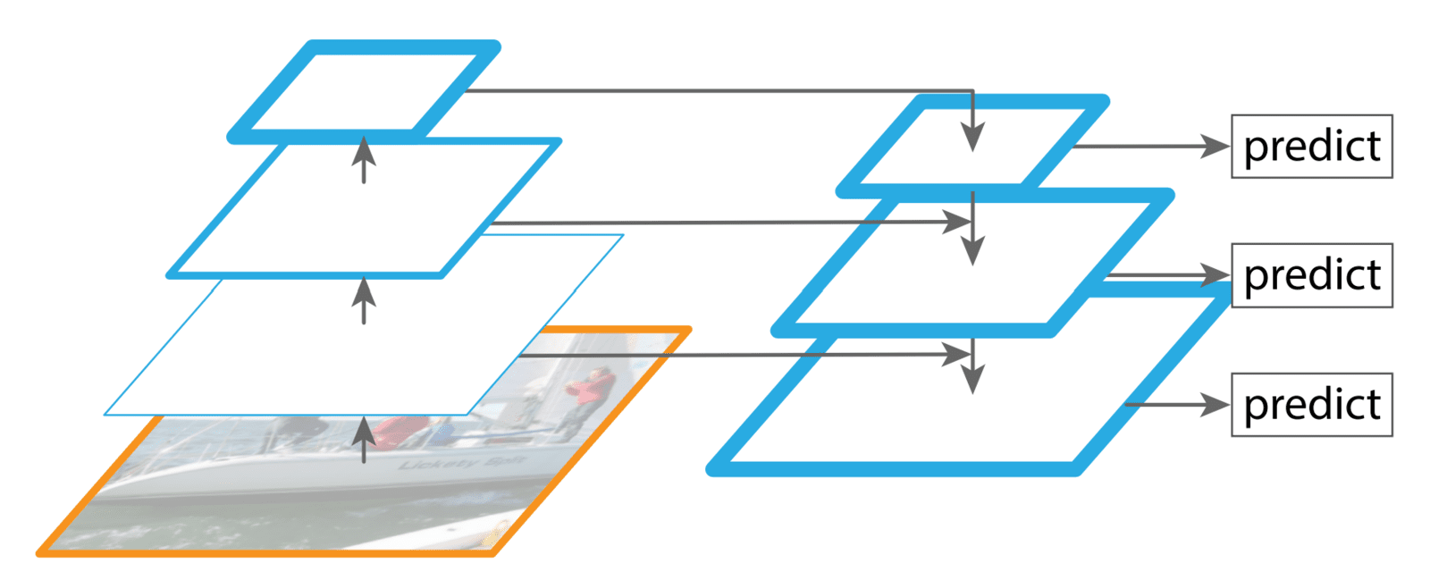
This can be easily understood by taking an example of feature pyramid networks. In FPN, predictions are made at different levels. Features from the higher and lower levels are merged so that refined semantically strong features can be combined with coarse and semantically weak features via a top-down pathway and lateral connections.
Objects of the same class may be present at different scales. Due to the continuous mixing and extraction of features, the sub-space representation of similar objects at different levels may no longer get mapped to similar locations in the kernel space. As an example, take figure (a) Without alignment, similar objects are no longer getting projected to the same space. This can be problematic.
To deal with this problem, we can perform addition and multiplication of output features and implicit representation. Doing so allows the kernel space to be translated, rotated, and scaled to align each output kernel space of neural networks. This makes the sub-space representation of similar objects from different levels to be aligned (figure (b) With alignment). This is how we can use (constant) implicit representations (vectors) to help with kernel space misalignment.
The authors mention that this technique can be helpful in knowledge distillation to integrate large and small models and handle the zero-shot domain transfer.
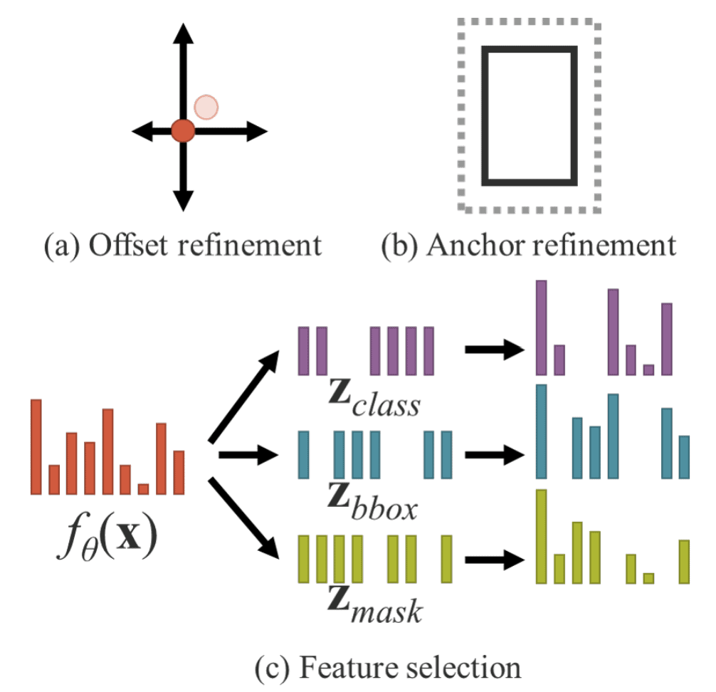
Formulation Of Implicit Knowledge In Unified Networks
In this section, we will discuss how implicit knowledge can be formulated in neural networks. The objective function of any conventional network training can be represented as follows:

Where the symbols represent:
- x: Observation
- theta θ: parameters of a neural network
- fθ: operation of the neural network
- epsilon ε: error term
- y: target of a given task
During training, the goal is to minimize the error term to make the neural network output as close as possible to the target. This is just a simpler way of saying that we want the observations belonging to the same target to be mapped to (preferably) the same location in the solution subspace. But in doing so, we create a network that is good at modeling a solution space discriminative for just a single task ti and invariant to other potential tasks T={t1, t1,.…, tn}.
The authors argue that this is problematic because to create a general-purpose neural network, we need to obtain representations that can serve all tasks belonging to T.
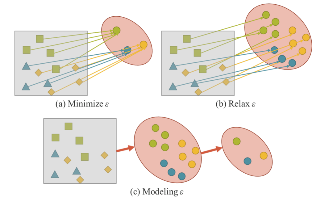
To do so, we need to (b) relax the error term ε so each task can find the information required.
But relaxing the error term can create mathematical problems. We wouldn’t be able to use simple operations such as argmax.
Instead, we can model the error term ε (c) to find solutions for different tasks. This means we want our network to generate more general sub-space representations (basically, learn how to relax the error term).
Excerpt from the paper:
“To train the proposed unified networks, we use explicit and implicit knowledge together to model the error term and then use it to guide the multi-purpose network training process.”
The corresponding equation for training is as follows:

Where,
- εex and εim: Operations that model the explicit and implicit errors from observation x and latent code z.
- g: Task-specific operation that combines or selects information from explicit and implicit knowledge.
The formulation can be simplified to:

The star * operator refers to possible ways to combine f and g.
How does it work during training and inference stage?
During the training phase, the authors assume that the model has no prior implicit knowledge and does not affect the explicit representations fθ(x). The initial prior is drawn from a normal distribution with parameters (µ, σ). When combining using the multiplication operator, we use µ=1, while for the other two, µ=0. The variance is kept very close to zero (0.02). z is a trainable tensor trained using the backpropagation algorithm.
During inference, as implicit knowledge is irrelevant to observation x, no matter how complex the implicit model g is, it can be reduced to a set of constant tensors before the inference phase is executed. In other words, the formation of implicit information has almost no effect on the algorithm’s computational complexity.
Paper Experiments
The authors chose to apply implicit knowledge to three aspects:
- Feature alignment for FPN
- Prediction refinement
- Multi-task learning
- Object detection
- Multi-label image classification
- Feature embedding.
The paper uses YoloV4-CSP as the baseline model. All the training hyper-parameters are compared to the default setting of Scaled-YoloV4.
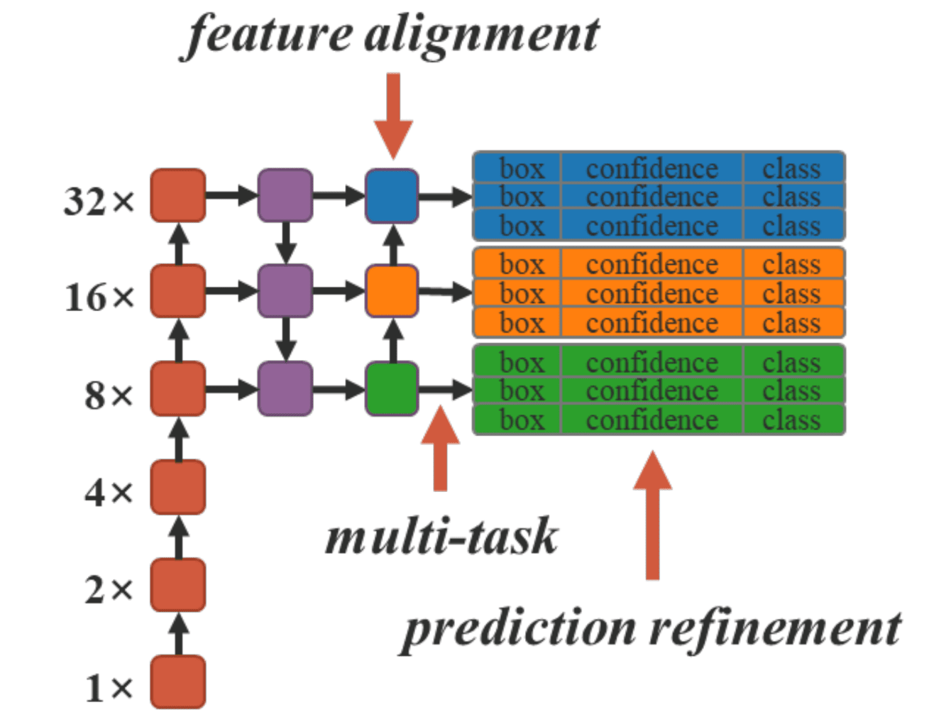
The authors have presented various ablation studies where they empirically prove that using implicit knowledge in conjunction with the explicit knowledge network does help to improve the results. You can go through them in the paper. The ones that stood out were:
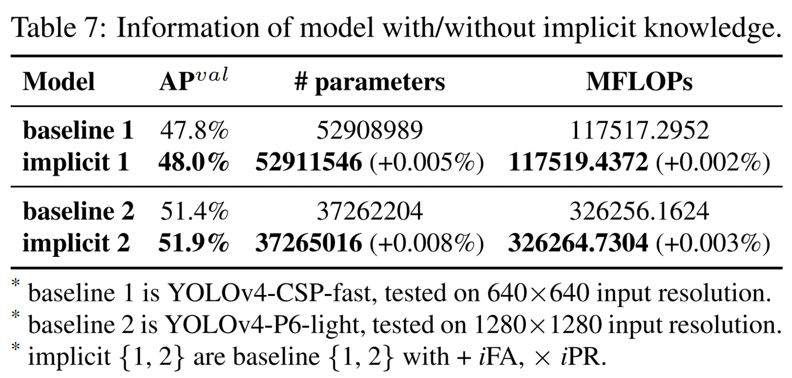
- Analysis of implicit models: It’s reported that the number of parameters and calculations increased by less than one ten-thousandth in the model with implicit knowledge. This can significantly improve the model’s performance, and the training process can converge quickly and correctly.
- Multi-task results: As highlighted in the previous sections, multi-task training is difficult and can often lead to degrading results. In the YoloR paper, the authors have provided results for two multi-task training scenarios: Joint Detection and Classification (JDC) and Joint Detection and Embedding (JDE).
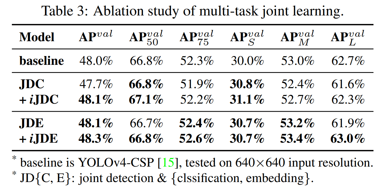
Take results for JDC as an example; when trained in a multi-task setting, the numbers indicate a significant performance drop. In contrast, the overall index score has increased significantly when the representation power is augmented by introducing implicit representation to each task branch. The performance of metrics, such as APval, AP50val, and APSval, surpasses that of a single-task training model. - The final experiment reported training and fine-tuning the object detection model using implicit knowledge for feature alignment and prediction refinement. The results are taken from their GitHub repository “paper” branch. A (better) new set of numbers is mentioned in the main branch, but their weights are unavailable.
| Model | Test Size | APtest | AP50test | AP75test | batch 1 throughput | FLOPS |
| YOLOR-P6 | 1280 | 54.1% | 71.8% | 59.3% | 76 fps | 326G |
| YOLOR-W6 | 1280 | 55.5% | 73.2% | 60.6% | 66 fps | 454G |
| YOLOR-E6 | 1280 | 56.4% | 74.1% | 61.6% | 45 fps | 684G |
| YOLOR-D6 | 1280 | 57.3% | 75.0% | 62.7% | 34 fps | 937G |
Note: There are four other models provided.
- In the main branch:
- YoloR-CSP
- YoloR-CSP-X
- In paper branch (small models ~18MB):
- YoloR-S4S2D
- YoloR-S4DWT
I’ll link additional details provided by the author in the references section.
After looking at these results, it’s tempting to train YoloR on a custom dataset and find out how much implicit knowledge helps with a custom task. Watch this space ⏳, as we have plans for this as well.
But the class of objects we want to detect is not limited to the COCO dataset. We want to be able to train these models for our own use cases as well.
Cheer Up!!! We’ve got you covered. We’ve recently released three excellent articles specifically for this task.
- The first post is about custom object detection training using YoloV5 models. The underlying codebase of YoloV5 makes it easy for anyone to perform. Recent Yolo models also use the codebase provided by YoloV5.
- In the second post, we perform custom training using YoloV6 on the Underwater trash dataset. The dataset is really tough, and YoloV6 does an outstanding job.
- The third post shows how to train and fine-tune YoloV7 models on real-world pothole detection datasets.
YoloR Object Detection Inference
Now, let’s get into the exciting part of this article: running inferences on videos using YoloR. Along with that, we will also compare results between YoloR and YoloV7 models.

YoloR PyTorch Code Setup
In the downloads, we have provided a ready-to-use Colab notebook that you can use to perform your own inference tests. We have also provided a jupyter notebook containing all the instructions and steps needed to run Yolor models locally.
- Clone the “paper” branch of the YoloR repository.
git clone -b paper https://github.com/WongKinYiu/yolor.git
- By default, the code requires PyTorch <=1.7.1, but we can get it to run with the latest versions with some minor changes. The source of error comes from the arguments passed to the Upsample module.
- In detect.py, at line 30, change the boolean value from
half= True tohalf = False - Find the
attempt_load(...)function in themodels/experimental.pyscript. Add the following code after line 140 (inside the for-loop)
- In detect.py, at line 30, change the boolean value from
if instance(m, nn.Upsample):
    m.recompute_scale_factor = None
That’s all the changes required for running YoloR with the latest version of PyTorch.
Download the following weights provided in the GitHub releases inside (create new) the “weights” folder in the cloned repo.
- yolor-p6-paper-541.pt
- yolor-w6-paper-555.pt
- yolor-e6-paper-564.pt
- yolor-d6-paper-573.pt
From the README file (paper branch), download the weights files weights for YoloR-S4DWT and YoloR-S4S2D from the drive links provided.
To run the YoloR-S4DWT model, some additional installation is required. Open a terminal in the cloned repository and run the following commands:
git clone https://github.com/fbcotter/pytorch_wavelets
cd pytorch_wavelets
pip install -r requirements.txt
pip install .
cd ..
To run inference, use the following command:
python detect.py --weights {weight_file_path} --source {source_video_path} --img-size {640|1280} --device {0 | cpu} --project {save root folder path} --name {save folder name} --exist-ok
The command line arguments are as follows
- –source: The path to the video file. This can also be an image or path to a directory containing multiple images and videos.
- –weights: The path to the weights file.
- –img-size: The frame size on which to run inference (use model specific).
- –device: The computation device. We can provide CPU or one digit from 0 to 3 indicating which GPU to use.
- –project: root save folder
- –name: The name of the output directory
That’s it.
YoloR Model Comparison
In this section, first, we’ll compare the inference speed between the two lightweight models on CPU and GPU.
The validation metrics for the two models are as follows:
| Model | Size | APval | AP50val | AP75val | APSval | APMval | APLval | FLOPS |
| YOLOR-S4S2D | 640 | 36.9% | 55.3% | 39.7% | 18.1% | 41.9% | 50.4% | 16G |
| YOLOR-S4DWT | 640 | 37.0% | 55.3% | 39.9% | 18.4% | 41.9% | 51.0% | 16G |
The two models are very similar to each other. Except for the difference in the first 3 backbone layers, the rest of the architecture is the same.
| YOLOR-S4DWT | YOLOR-S4S2D |
Backbone: [-1, 1, DWT, []], # 0 | Backbone: [-1, 1, ReOrg, []], # 0 |
Where,
- DWT – Discrete wavelet transform
- S2D- Spatial to Depth (re-organization)

Run command:
python detect.py --weights weights\{yolor-ssss-dwt.pt | yolor-ssss-s2d.pt} --source videos\video_1.mp4 --img-size 640 --device {0 | cpu} --project inference_tests --name small_models --exist-ok
The metrics table shows that both models have very comparable metrics, which is also evident from the above video. The models also have very similar inference speeds on both GPU and CPU.
Next, let’s run inference for all 4 major YoloR variants.
From the video, it’s easily discernible that all larger models (trained on 1280 size ) are better than the smaller versions (as they should be). In the bigger versions, the models can properly detect the car on the right side across the pillar as one, as well as the missed dog detection or detecting dog as a handbag (from the beginning).
Another comparison between the smallest and the largest model
We can clearly see the superiority of the largest model over the lightweight variant.
YoloR vs YoloV7 – Inference & Detection Quality Comparison
As mentioned before, the team behind YoloR and YoloV7 are the same. So we can expect YoloV7 to be at least on par, if not better, than YoloR.
The first comparison between YoloR-S4-Dwt and YoloV7-tiny on GPU.
| Model | Size | APval | AP50val | AP75val | APSval | APMval | APLval | FLOPS |
| YOLOR-S4DWT | 640 | 36.9% | 55.3% | 39.7% | 18.1% | 41.9% | 50.4% | 16G |
| YoloV7-tiny | 320 | 30.8% | 47.3% | 32.2% | 10.0% | 31.9% | 52.2% | 3.5G |
YoloV7-tiny is much smaller than YoloR-S4-DWT. The YoloV7-tiny model detects the Alaskan Malamute (dog) as a cow. But the inference speed of the tiny model is ~2.4 times of YoloR-S4-DWT.
Next up, we have the inference results of the big models.

First, we compare YoloR-E6 with the YoloV7-E6 Video YoloR-E6 variant, which is bigger than V7-E6.
Apart from minor differences in classification threshold, the detection results of both models are very close to each other. But, in terms of inference speed, YoloV7-E6 is the clear winner.
Next, we compared the results of the best models: YoloR-D6 vs. YoloV7-E6E
This is interesting because both models are really close to each other in terms of being the SOTA in the Real-time object detection category. Their detection accuracy for people, cars, trucks, and buses is close. But they both made the same error in detecting the petrol pump as a truck. This, I believe, is a limitation due to the dataset used for training. The scale and orientation of objects captured from a height differ from those seen from approximately a leveled surface.
We get similar results on another drone footage where the parked cars are detected as cell phones.
From the above results, we can partially conclude that the YoloR and YoloV7 are in direct competition with each other. Though YoloV7 may seem the better option to explore in the aftermath, the contributions of YoloR are not to be taken lightly.
After developing YoloR, the authors created YoloV7, which explains why YoloV7 has better inference speed and (same or better) results than YoloR models.
Currently, YoloV5, YoloV6, and YoloV7 are in competition 🏁 with each other to be the best real-time object detection model.
🤔 Intrigued by this? We were as well. So, we also did a comparative analysis of YoloV5, YoloV6 and YoloV7 to help you further understand the difference between the new models and help you choose the best for your project.
Summary
YoloR is the 9th object detection model in the Yolo series. The authors have taken the Yolo approach and have improved the object detection algorithm in many ways.
In this article📜, we covered a comprehensive list of topics related to YoloR. To summarise.
- We started with establishing YoloR place in the entire Yolo series.
- In-depth exploration of the fundamental difference between YoloR and other Yolo series models.
- Deep dive into the basic intuition of YoloR using multiple examples for better understanding.
- Exploratory route to understanding the key architectural changes in YoloR and how the new additions fit into the architecture.
- Investigated the usefulness of implicit knowledge in neural networks.
- Finally, we examined the key results published in the paper and compared YoloR with models with each other and YoloV7.
We would love to hear from you. Please feel free to ask questions in the comment section; we are more than happy to converse with you.
🌟Happy learning!
References
- Paper – Yolo Only Learn One Representation
- GitHub – YoloR
- GitHub issues – How do I use YoloR-SSSS-DWT model?
- GitHub issues – What’s differs ImplicitA and ImplicitC in layers.py
- YoloR-CSP and YoloR-CSP-X








100K+ Learners
Join Free OpenCV Bootcamp3 Hours of Learning