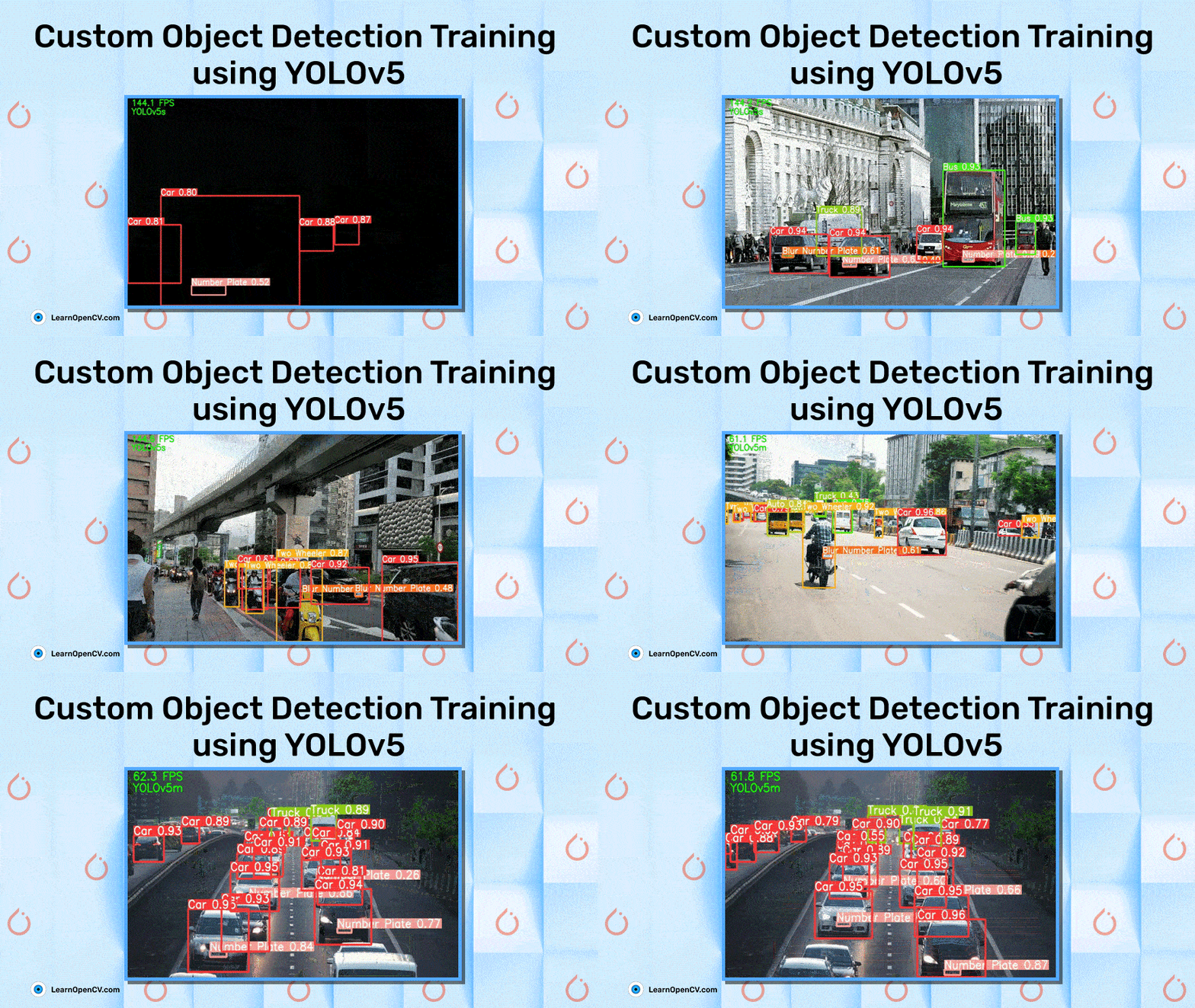
In this article, we are fine tuning YOLOv5 models for custom object detection training and inference.
- Introduction
- What is YOLOv5?
- Custom Object Detection Training using YOLOv5
- The Custom Training Code
- Performance Comparison
- Conclusion
Introduction
The field of deep learning started taking off in 2012. Around that time, it was a bit of an exclusive field. We saw that the people writing deep learning programs and software were either deep learning practitioners, researchers with extensive experience in the field, or people with excellent coding skills.
Today, only after 10 years or so, the scene has changed drastically, and for the better. Literally, a student who has been learning deep learning for only a few weeks can train a neural network model within 20 lines of code. And not just off-the-shelf training on benchmark datasets. We are talking about training on custom datasets with some of the best models out there. Not believing it? Well, this is exactly what we will do in this post with Custom Object Detection Training using YOLOV5.
We will cover the following points in this blog post:
- We will train YOLOv5s (small) and YOLOv5m (medium) models on a custom dataset.
- We will also check how freezing some of the layers of a model can lead to faster iteration time per epoch and what impacts it can have on the final result.
- Along with that, we will compare the performance of the models, which include the mAP, FPS, and the inference time on CPU and GPU.
YOLO Master Post – Every Model Explained
Don’t miss out on this comprehensive resource — Mastering All Yolo Models for a richer, more informed perspective on the YOLO series.
What is YOLOv5?
If you have been in the field of machine learning and deep learning for some time now, there is a very high chance that you have already heard about YOLO. YOLO is short for You Only Look Once. It is a family of single-stage deep learning-based object detectors. They are capable of more than real-time object detection with state-of-the-art accuracy.
Officially, as part of the Darknet framework, there are four versions of YOLO. Starting from YOLOv1 to YOLOv4. The Darknet framework is written in C and CUDA.
YOLOv5 is the next version equivalent in the YOLO family, with a few exceptions.
- The project was started by Glenn Jocher under the Ultralytics organization on GitHub.
- It was written using Python language, and the framework used is PyTorch.
- It is in itself a collection of object detection models. From tiny models capable of giving real-time FPS on edge devices to huge and accurate models meant for cloud GPU deployments. It has almost everything one might need.

It has a host of other features and capabilities which make it the choice of go-to object detection model/repository when anybody even thinks of object detection today. We will check those out shortly.
Models Available in YOLOv5
To begin exploring the entire landscape of YOLOv5, let’s start with the models. It contains 5 models in total. Starting from YOLOv5 nano (smallest and fastest) to YOLOv5 extra-large (the largest model).
The following is a short description of each of these:
- YOLOv5n: It is a newly introduced nano model, which is the smallest in the family and meant for the edge, IoT devices, and with OpenCV DNN support as well. It is less than 2.5 MB in INT8 format and around 4 MB in FP32 format. It is ideal for mobile solutions.
- YOLOv5s: It is the small model in the family with around 7.2 million parameters and is ideal for running inference on the CPU.
- YOLOv5m: This is a medium-sized model with 21.2 million parameters. It is perhaps the best-suited model for many datasets and training as it provides a good balance between speed and accuracy.
- YOLOv5l: It is the large model of the YOLOv5 family with 46.5 million parameters. It is ideal for datasets where we need to detect smaller objects.
- YOLOv5x: It is the largest among the five models and has the highest mAP among the 5 as well. Although it is slower compared to the others and has 86.7 million parameters.
The following figure shows an even better overview of all the models, including the inference speed on CPU, GPU, and also the number of parameters with an image size of 640.
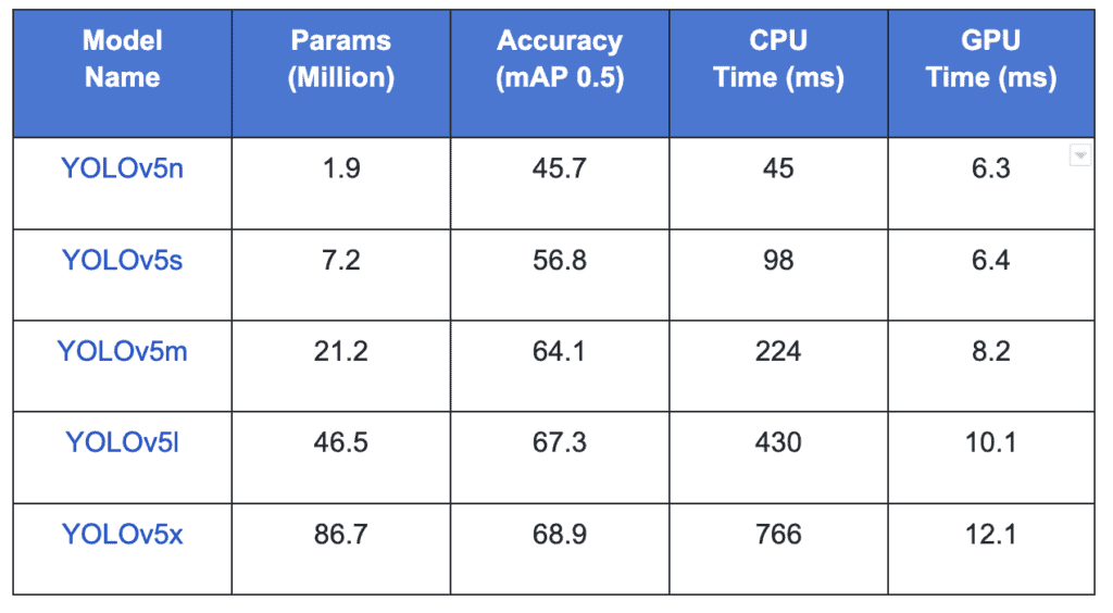
All the model checkpoints are available for download from the Ultralytics YOLOv5 repository. They have been pretrained on the MS COCO dataset for 300 epochs.
Features Provided by the YOLOv5 Repository and Codebase
If you go through the repository, it becomes pretty evident that it makes training and inference on custom datasets extremely easy. So much so that it is safe to say if you already have a dataset ready in the correct format, you can get started with training within 2 minutes.
But training and inference are not all. It contains a lot of other features which make it really special. Let’s go over them.
A Number of Models to Choose From
We have already discussed above that we can choose from 5 different models depending on our use case and dataset. Whether it is training a real-time detector for the edge or deploying a state-of-the-art object detection model on cloud GPUs, it has everything one might need.
Numerous Export Options
Only training and inference of models are not enough for an object detection pipeline to be complete. In real-life use cases, deployment is also a major requirement. Before deployment, we mostly need to convert (export) the trained model to the correct format.
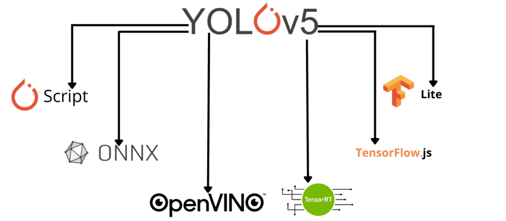
We can convert the native PyTorch (.pt) models to formats like:
- TorchScript
- ONNX
- OpenVINO
- TensorRT
- CoreML
- TensorFlow SavedModel, GraphDef, Lite, Edge TPU, and TensorFlow.js as well.
Complement your learning with practical applications in our article ‘Object Detection using YOLOv5 OpenCV DNN in C++ and Python,’ which covers the implementation of YOLOv5 using the OpenCV DNN module.
This opens a myriad of deployment options for any deep learning engineer.
Logging
YOLOv5 repository provides TensorBoard and Weights&Biases logging by default. Although you may need to create a Weights&Biases account and provide the API credentials before you can start the training for proper logging.
Even if you skip that, TensorBoard logs are already present, containing every metric, loss, and image along with all the validation predictions. This makes it easier for us to take a look at the performance metrics at any point after training a model.
Genetic Algorithm for Anchor Box Selection
While many object detection models use predefined anchor boxes according to the MS COCO dataset, YOLOv5 takes a different approach. In fact, the previous versions of YOLO, like YOLOv2 used only k-Means clustering for that.
But YOLOv5 uses a genetic algorithm to generate the anchor boxes. They call this process autoanchor, which recomputes the anchor boxes to fit the data if the default ones are not good. This is used in conjunction with the k-Means algorithm to create k-Means evolved anchor boxes. This is one of the reasons why YOLOv5 works so well, even on varied datasets.
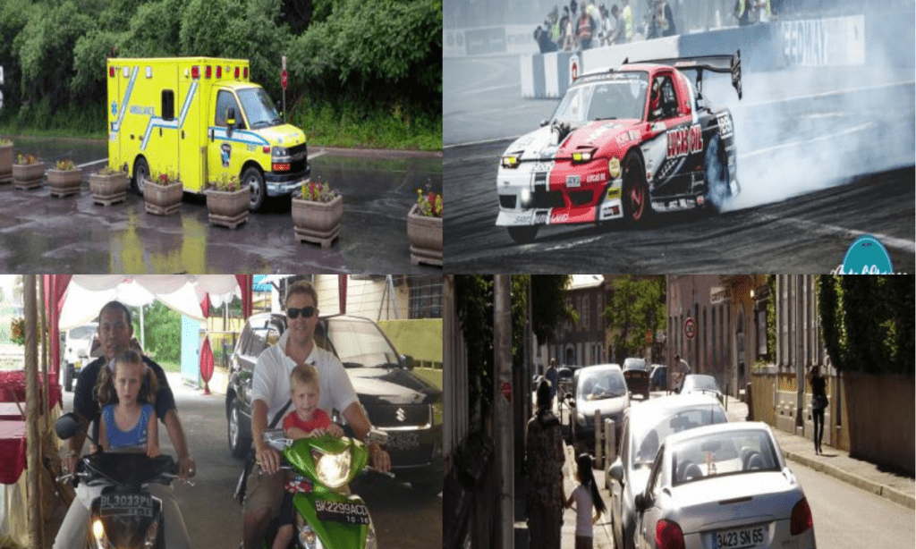
Mosaic Augmentation
Another reason for such good training and detection results of the YOLOv5 model is mosaic augmentation.
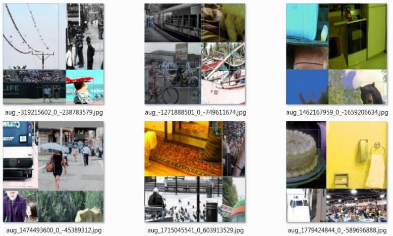
Caption: An example of mosaic augmentation (image source).
In simple words, it combines 4 different images into one so that the model can learn to deal with varied and difficult images. It uses other augmentation techniques also, along with mosaic augmentation.
Comparison Between YOLOv5 and YOLOv3
Now that we have seen the different models available in YOLOv5 and what are the different features the codebase provides, let’s compare YOLOv5 with the previous YOLOv3 models. These comparisons mostly focus on the mAP of the models with 608×608 image dimensions and include both Darknet and Ultralytics models.
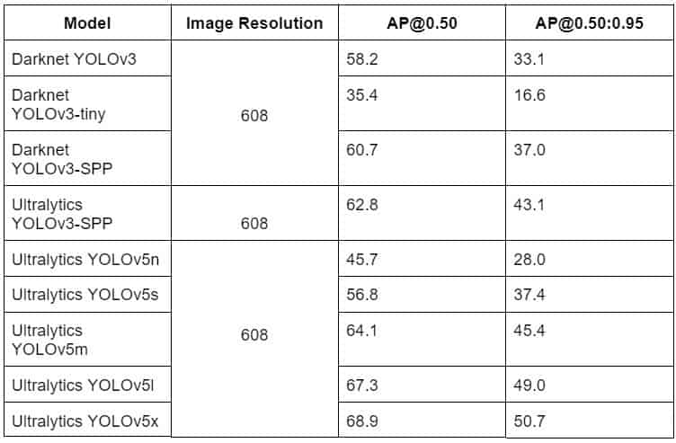
It is clear that the Ultralytics YOLOv3-SPP model was able to beat the Darknet YOLOv3 SPP model in terms of mAP. And the Ultralytics YOLOv5 models perform even better. The YOLOv5m, which is roughly a 21 million parameter model, is able to beat the YOLOv3-SPP model, which is a 63 million parameter model. This shows how much the Ultralytics models have improved over the years.
Note: In the above figure, you may find that some of the Darknet YOLOv3 results are slightly better compared to the original paper. The reason is that, as the Darknet YOLOv3 models were updated, the mAP numbers were updated by Ultralytics in their repository as well. This also allows us to have a fair comparison among all the last updated models.
The new YOLOv6 model makes many fundamental changes to the backbone, neck, and head compared to YOLOv5. Don’t miss out on the details and see how it compares to the other YOLO models.
Custom Object Detection Training using YOLOv5
In this article for custom object detection training using YOLOv5, we will use the Vehicle-OpenImages dataset from Roboflow.
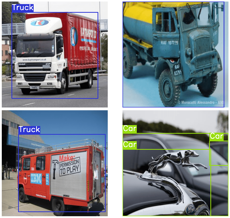
The dataset contains images of various vehicles in varied traffic conditions. These images have been collected from the Open Image dataset. The images are from varied conditions and scenes. It contains 5 classes in total. They are Car, Bus, Motorcycle, Truck, Ambulance.
The dataset contains images of 5 different types of vehicles in varied conditions. Such a dataset with these classes can make for a good real-time traffic monitoring application. Although we are not going to do that in this post, we will be completing the first step required in such a process. That is, building a good object detector. And with YOLOv5, it will be really easy as the dataset is already in the required format.
The dataset contains 439 images for training, 125 images for validation, and 63 images for testing. But we will only use the training and validation sets in this post. Before moving forward, here are a few images with the ground truth boxes drawn on them.
Approach for Custom Training
Let’s check out what we will cover during the custom training using YOLOv5.
- We will start with training the small YOLOv5 model.
- Then we will train a medium model and check the improvement as compared to the small model.
- Next, we will freeze a few layers of the medium model and train the model again.
- We will carry out inference in all the above cases and also compare the mAP metrics along with the FPS during inference on videos.
The Custom Training Code
Let’s get started with the coding part. All the code is part of a Jupyter notebook that you can access from the download section.
Here, we will go through all the necessary and important coding parts. These include:
- The dataset preparation.
- Training of the three models as discussed above.
- Performance comparison.
- Inference on images and videos.
Let’s go over all the important parts of the code, starting with importing the modules and libraries that we use in the notebook.
import os
import glob as glob
import matplotlib.pyplot as plt
import cv2
import requests
We will need glob for capturing file paths in a directory, matplotlib for visualization, and cv2 for reading images.
Next, we define a few constants and hyperparameters.
TRAIN = True
# Number of epochs to train for.
EPOCHS = 25
Above, we have a boolean called TRAIN. If this is True, then running the code will train all three models in the notebooks. If we provide the value as False, then if any previously trained model is present in the result directory, it will be used for inference. This is a good measure to ensure that we need not train all the models each time if we want to carry out inference.
Helper Function to Download Files
The following function is for downloading any file in the notebook. Further on, we will use it for downloading the inference dataset.
def download_file(url, save_name):
    url = url
    if not os.path.exists(save_name):
        file = requests.get(url)
        open(save_name, 'wb').write(file.content)
    else:
        print('File already present, skipping download...')
Preparing the Dataset
The next step is downloading and preparing the dataset. We need a simple helper function for downloading the dataset and extract.
if not os.path.exists('train'):
    !curl -L "https://public.roboflow.com/ds/xKLV14HbTF?key=aJzo7msVta" > roboflow.zip; unzip roboflow.zip; rm roboflow.zip

    dirs = ['train', 'valid', 'test']

    for i, dir_name in enumerate(dirs):
        all_image_names = sorted(os.listdir(f"{dir_name}/images/"))
        for j, image_name in enumerate(all_image_names):
            if (j % 2) == 0:
                file_name = image_name.split('.jpg')[0]
                os.remove(f"{dir_name}/images/{image_name}")
                os.remove(f"{dir_name}/labels/{file_name}.txt")
The above code downloads the dataset into the current directory if it is not already present and extracts it. The original data had two instances of each image and label file. The rest of the code in the above block deletes the duplicate image and its corresponding text file containing the label.
It is also important to know the directory structure of the dataset before using it for training.
├── test
│   ├── images
│   └── labels
├── train
│   ├── images
│   ├── labels
│   └── labels.cache
├── valid
│   ├── images
│   ├── labels
│   └── labels.cache
├── data.yaml
├── README.dataset.txt
└── README.roboflow.txt
We have the images and labels in their respective folder. As discussed earlier, we will use the train and valid folders for the YOLOv5 custom object detection training..
The YAML File
Perhaps one of the most important properties of YOLOv5 training is the dataset YAML file. This file contains the path to the training and validation data, along with the class names. While executing the training script, we need to provide this file path as an argument so that script can identify the image paths, the label paths, and also the class names. The dataset already contains it. The following is the content of the data.yaml file that we use for training here.
train: ../train/images
val: ../valid/images
nc: 5
names: ['Ambulance', 'Bus', 'Car', 'Motorcycle', 'Truck']
Note: All the paths in the above file should be relative to the training script. As we will be executing the scripts inside the yolov5 directory after cloning it, therefore, we have given the value of the train and valid paths as “../train/images” and ../valid/images, respectively.
Clone the YOLOv5 Repository
For using any of the functionalities of the YOLOv5 codebase, we need to clone their repository. The next few lines of code clone the repository, enter into the yolov5 directory and install all the requirements that we may need for running the code.
if not os.path.exists('yolov5'):
    !git clone https://github.com/ultralytics/yolov5.git
%cd yolov5/
!pip install -r requirements.txt
If everything runs smoothly, you should see a successful installation of all the requirements.
Training using YOLOv5 Models
If you remember, we discussed how if we have the dataset ready with us, we can start the training right away. Actually, we are in that state now. If we execute the train.py script with the path to the data.yaml file, the training will start immediately. The script will choose all the default parameters available for training.
But we will take a slightly different approach. We will control the training arguments as per our requirement. We will run the training script three different times, all with slightly different arguments.
Note: All the training and inference experiments were carried out on a machine with an 8th generation i7 CPU, 6 GB GTX 1060 GPU, and 16 GB of RAM.
Training the Small Model (yolov5s)
We will be starting with training all the layers of the small model. This means that, although the pretrained weights will be loaded, the entire model will be fine-tuned on the new dataset.
And frankly, even with controlling all the arguments, it is just one simple command as shown below.
RES_DIR = set_res_dir()
!python train.py --data ../data.yaml --weights yolov5s.pt \
    --img 640 --epochs {EPOCHS} --batch-size 16 --name {RES_DIR}
Okay! Let’s go through everything that is happening in the above code block.
First, we are creating a new directory for saving the results. The path for that is saved in the RES_DIR variable. You will find the entire function definition for set_res_dir in the notebook. This is important because we want to control where the results are saved. Else, the script will create its own directories as run_1, run_2, and so on, while executing the train.py script.
Now, let’s go over all the arguments of the training script.
--data: This accepts the path to the dataset YAML file that we created earlier. In our case, it is one directory back to the current directory, and that’s why it is../data.yaml.--weights: This argument accepts the model which we want to use for training. As we are using the small model from the YOLOv5 family, the value isyolov5s.pt.--img: We can also control the image size while training. The images will be resized to this value before being fed to the network. We are resizing them to 640 pixels which are also the most common ones used.--epochs: This argument is used to specify the number of epochs. As we have already specified the number of epochs in theEPOCHSvariable above, we provide that here.--batch-size: This is the number of samples that will be loaded into one batch while training. Although the value is 16 here, you can change it according to the GPU memory that is available.--name: We can provide a custom directory name where all the results will be saved. In our case, we provide a path that we just created by calling theset_res_dirfunction.
After executing the above code, the training will begin, and it will take some time, depending on the hardware. It is highly recommended that you run all the training on a GPU.
If the training completes successfully, then you will see an output similar to the following.
Epoch   gpu_mem       box       obj       cls    labels  img_size
      0/24     3.48G    0.1009   0.03861   0.04645        26       640: 100%|███
               Class     Images     Labels          P          R     mAP@.5 mAP@
                 all        125        227      0.149      0.211     0.0944     0.0305
...
Epoch   gpu_mem       box       obj       cls    labels  img_size
     24/24     3.94G   0.03121   0.01958  0.009307        21       640: 100%|███
               Class     Images     Labels          P          R     mAP@.5 mAP@
                 all        125        227      0.655      0.515      0.587       0.41

25 epochs completed in 0.190 hours.
Optimizer stripped from runs/train/results_4/weights/last.pt, 14.5MB
Optimizer stripped from runs/train/results_4/weights/best.pt, 14.5MB

Validating runs/train/results_4/weights/best.pt...
Fusing layers...
Model summary: 213 layers, 7023610 parameters, 0 gradients
               Class     Images     Labels          P          R     mAP@.5 mAP@
                 all        125        227      0.514      0.646      0.588       0.41
           Ambulance        125         32      0.541      0.812      0.741      0.605
                 Bus        125         23      0.586      0.739      0.714      0.502
                 Car        125        119      0.521       0.58      0.531       0.34
          Motorcycle        125         23      0.668      0.699      0.659      0.397
               Truck        125         30      0.254        0.4      0.296      0.204
The YOLOv5s model was able to achieve an mAP of 58.8% at 0.5 IoU and 41% at 0.5:0.95 IoU.
The following figure shows the results.png file containing all the losses and mAP in the current result directory.
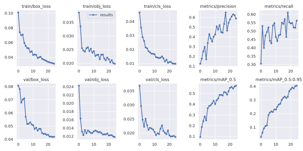
Loss and mAP results after training the YOLOv5s model for 25 epochs.
All things considered, for a model with around 7 million parameters, these results are not bad at all. In fact, the whole training took around 12 minutes on a mid-range GPU. Also, in the end, you can see it shows the custom directory where all the results are saved.
The Validation Predictions and Inference for YOLOv5s
During training, the codebase saves the predictions from the validation batches on each epoch to the result directory. Before we can check those out, let’s write a helper function to find all the validation predictions in a result directory and show them.
# Function to show validation predictions saved during training.
def show_valid_results(RES_DIR):
    !ls runs/train/{RES_DIR}
    EXP_PATH = f"runs/train/{RES_DIR}"
    validation_pred_images = glob.glob(f"{EXP_PATH}/*_pred.jpg")
    print(validation_pred_images)
    for pred_image in validation_pred_images:
        image = cv2.imread(pred_image)
        plt.figure(figsize=(19, 16))
        plt.imshow(image[:, :, ::-1])
        plt.axis('off')
        plt.show()
The above function accepts the result directory path. We can visualize the images as follows.
show_valid_results(RES_DIR)
Here are a few of those results.

It looks like even the small model is capable of giving pretty good results. Although it is worthwhile to note that it is not able to detect the car in the first image. Apart from that, it is capable of detecting the objects in all other images.
Moving on to the inference part. Here, we need a few helper functions as well. These are the functions that directly use the inference script. So, it is pretty important to know about them. Also, we will reuse these functions further on as we train the medium model.
# Helper function for inference on images.
def inference(RES_DIR, data_path):
    # Directory to store inference results.
    infer_dir_count = len(glob.glob('runs/detect/*'))
    print(f"Current number of inference detection directories: {infer_dir_count}")
    INFER_DIR = f"inference_{infer_dir_count+1}"
    print(INFER_DIR)
    # Inference on images.
    !python detect.py --weights runs/train/{RES_DIR}/weights/best.pt \
    --source {data_path} --name {INFER_DIR}
    return INFER_DIR
The inference function can be used for carrying out inference on images and videos when provided with the result directory path where the model is saved and the data path where the images/videos are present. Each time this function will create a new inference directory to save the results.
But the most important part here is the detect.py script that runs the inference. Going over the arguments will provide us with more insight into its working.
--weights: This argument is used to provide the path to the trained weights to be used for inference. And if you observe each time properly, we are using the best model, that isbest.pt.--source: We need to provide the path where the images or videos are present.--name: Finally, each time, we use a custom directory to save the inference results to easily keep track of the results.
One thing to note here is that we use the same detect.py script for inference on images and videos. The same detection script can run inference on both images and videos by checking the file extension and calling the appropriate methods.
There is just one final helper function for visualizing the inference images stored on the disk after running detect.py. This will help us visualize the results directly in the Jupyter Notebook.
def visualize(INFER_DIR):
# Visualize inference images.
    INFER_PATH = f"runs/detect/{INFER_DIR}"
    infer_images = glob.glob(f"{INFER_PATH}/*.jpg")
    print(infer_images)
    for pred_image in infer_images:
        image = cv2.imread(pred_image)
        plt.figure(figsize=(19, 16))
        plt.imshow(image[:, :, ::-1])
        plt.axis('off')
        plt.show()
Now, we can entirely focus on the inference and check out the results. Let’s start with the image inference using the trained YOLOv5s model and visualizing them.
# Inference on images.
IMAGE_INFER_DIR = inference(RES_DIR, 'inference_images')
visualize(IMAGE_INFER_DIR)
The following figure shows the image inference results.
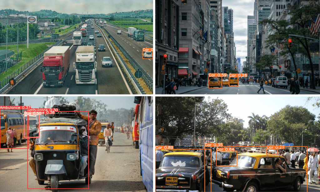
The limitations and strengths of the small model are pretty evident from here. Starting clockwise, It is only able to detect one car in the first image. Also, it is detecting the buses wrongly as Ambulance in the last image.
Nowadays, even smaller YOLO models tend to perform better when fine tuning even on difficult datasets. The results of fine tuning YOLOv7 on the pothole datasets is good proof of this.
Next, we will run inference on videos by executing the video_inference function.
inference(RES_DIR, 'inference_videos')
Let’s check out one of the inference results here.
It seems like the YOLOv5s model is missing a few detections, especially on the other side of the road. Also, there is a bit of fluctuation in the detections. But we don’t really have a comparison yet.
On the GTX 1060 GPU, the average time taken per frame was around 8 milliseconds which amounts to 125 FPS. The FPS is quite good, considering the predictions that we got here.
Training a YOLOv5 Medium Model
It’s time to train the medium model now. Training this will also allow us to compare the model’s results with the previous ones.
We will use the same training script while providing the new model name only.
RES_DIR = set_res_dir()
if TRAIN:
    !python train.py --data ../data.yaml --weights yolov5m.pt \
    --img 640 --epochs {EPOCHS} --batch-size 16 --name {RES_DIR}
The medium model took around 30 minutes to train for 25 epochs. The following are the final mAP results.
Model summary: 290 layers, 20869098 parameters, 0 gradients
               Class     Images     Labels          P          R     mAP@.5 mAP@
                 all        125        227       0.67      0.601       0.66      0.468
           Ambulance        125         32      0.748      0.781       0.85      0.691
                 Bus        125         23      0.655      0.696      0.654       0.48
                 Car        125        119      0.651      0.579      0.606      0.419
          Motorcycle        125         23      0.714      0.651       0.78      0.436
               Truck        125         30      0.583        0.3      0.409      0.316
The medium model results are considerably better. The mAP at 0.5 IoU is 66.0% which is obviously higher than the small model.
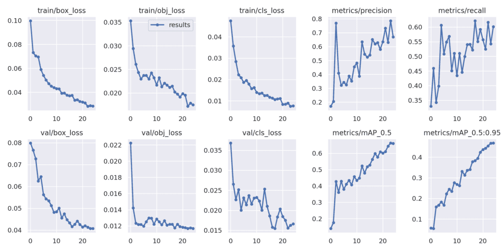
Also, the decrease in the loss looks much more stable in this case.
Now, let’s take a closer look at the image inference results here.

The improvement in the inference result is quite obvious from the above figure. It can detect more vehicles and with more confidence. But as you may observe, it still detects some of the buses and trucks as Ambulance. Surely, more training will lead to better results.
And following is the video inference result on the same video as above for comparison. The medium model can detect more vehicles with better confidence. Also, observe that the model is now able to detect the vehicles which are far off and were missed by the small model.
Even the medium model seems to run at an impressive 62 FPS on the GTX 1060 GPU with much more improved results. This is more than real-time speed with really good predictions.
Training Medium YOLOv5 Model by Freezing Layers
In object detection, we generally use models which are pretrained on the MS COCO dataset and fine-tune them on our own dataset. Most of the time, we train all the layers of the model, as object detection is a challenging problem to solve with large variations in datasets.
But we need not always train the entire model. Pretrained models are pretty powerful, and we can achieve almost the same result by freezing some layers and training the others. The only problem is that it is not very straightforward to do so. We often need to tinker with the source code to freeze layers.
But Ultralytics YOLOv5 makes it really easy to freeze a few layers of the model and train the others. We need to use the --freeze argument while executing the train.py script.
Let’s train the model now and check whether any of our above theories are true.
RES_DIR = set_res_dir()
if TRAIN:
    !python train.py --data ../data.yaml --weights yolov5m.pt \
    --img 640 --epochs {EPOCHS} --batch-size 16 --name {RES_DIR} \
    --freeze 0 1 2 3 4 5 6 7 8 9 10 11 12 13 14
The YOLOv5 medium model has 25 blocks in total (from 0 to 24). Each block is a stacking of different layers. When we freeze the first 15 blocks, then the convolutional and batch normalization weights are frozen. If you take a look at the output before the training starts, you will see output similar to the following.
freezing model.0.conv.weight
freezing model.0.bn.weight
freezing model.0.bn.bias
.
.
.
freezing model.14.conv.weight
freezing model.14.bn.weight
freezing model.14.bn.bias
Here, model.# indicates the block number and then the layer type. As we can see, all the convolutional and batch normalization weights from blocks 0 to 14 are frozen. That leaves only 10 more trainable blocks.
The following block shows the results after training for 25 epochs.
Model summary: 290 layers, 20869098 parameters, 0 gradients
               Class     Images     Labels          P          R     mAP@.5 mAP@
                 all        125        227      0.578      0.669       0.64      0.456
           Ambulance        125         32       0.65      0.812      0.805       0.64
                 Bus        125         23      0.569      0.783      0.712      0.547
                 Car        125        119      0.503      0.586      0.545      0.364
          Motorcycle        125         23      0.753      0.665      0.684      0.412
               Truck        125         30      0.418        0.5      0.453      0.318
The mAP values are higher than both YOLOv5s fully trained but slightly lower than the fully trained medium model. The results are also pretty good here.
Moreover, check out these image inference results.
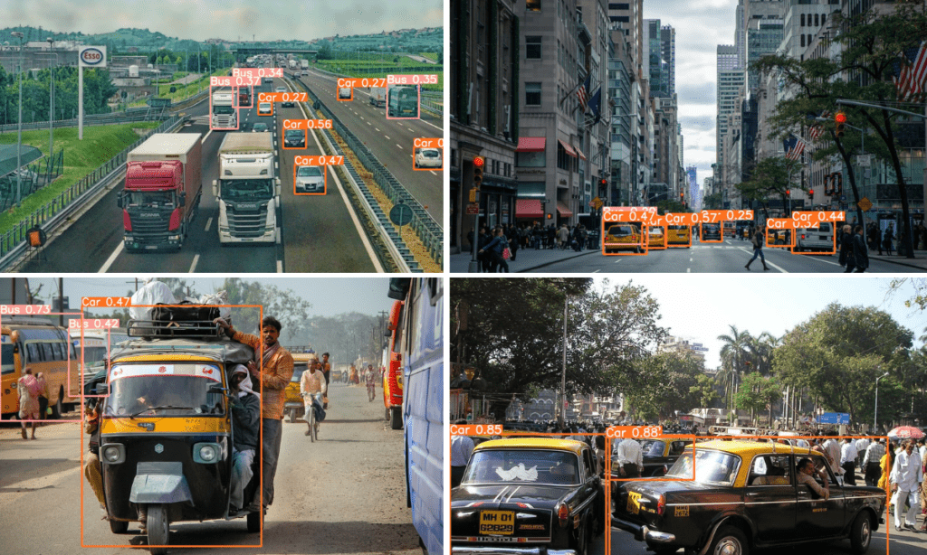
Interestingly, for some of the objects, these results are much better compared to the previous two inferences. But the model is still missing out on the trucks for the first image.
Running the video inference will give the same FPS, as the number of layers is not affected during inference. This experiment showed us that, if necessary, we can achieve just as good results by freezing some of the layers and shortening the training time.
Benefits of Training by Freezing Layers
From the above experiment, we can right away mention a few benefits of freezing a few layers and training the model.
- First, as we are freezing a few layers, those layers do not get trained, and backpropagation does not happen through those layers. This means that the training iteration time decreases. It is quite evident from the above training as well, which took only 15 minutes to complete compared to the 30 minutes of the full medium model training.
- Second, even though we froze a few blocks, the medium model is still more than capable of generating predictions just as good as that of a fully trained model. We could see in the above inference results the predictions were better than the small model.
Performance Comparison
This section contains the performance comparison graphs of all models, which include the following:
- Training time.
- Mean Average Precision.
- Inference speed on GPU.
- Inference speed on CPU.
Training Time Comparison
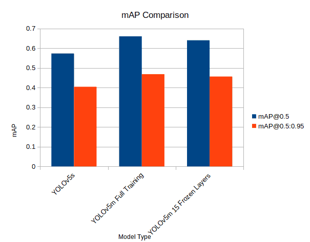
mAP Comparison

Inference Speed
Here is the average inference speed on videos for all three models.
Hardware used: Intel i7 8th gen laptop CPU, 6 GB GTX 1060 laptop GPU.
| Model Type | GPU Inference Speed in ms (FPS) | CPU Inference Speed in ms (FPS) |
| YOLOv5s | 8.0 ms (125 FPS) | 55 ms (18 FPS) |
| YOLOv5m Full Training | 16 ms (62 FPS) | 133 ms (7.5 FPS) |
| YOLOv5m Frozen Layers | 16 ms (62 FPS) | 133 ms (7.5 FPS) |
Further explore YOLOv5’s capabilities in our guide Getting Started with YOLOv5 Instance Segmentation, perfect for those looking to delve into advanced segmentation techniques.
Conclusion
We carried out a lot of training and inference experiments using YOLOv5 in this post. We started with custom object detection training and inference using the YOLOv5 small model. Then we moved to the YOLOv5 medium model training and also medium model training with a few frozen layers. This post gave us good insights into the working of the YOLOv5 codebase and also the performance & speed difference between the models.
Given the sheer amount of experiments carried out in this post, did you realize one thing? We did not write a single line of deep learning code except a few generic Python functions. This shows how accessible the field of deep learning is becoming, and hopefully, it will move in the same direction in the future as well. If you try custom training on your own dataset and find something interesting, don’t forget to share your results in the comment section.


100K+ Learners
Join Free OpenCV Bootcamp3 Hours of Learning