YOLO11 is finally here, revealed at the exciting Ultralytics YOLO Vision 2024 (YV24) event. 2024 is a year of YOLO models. After the release of YOLOv8 in 2023, we got YOLOv9 and YOLOv10 this year, and now YOLO11. You might think like another day, another YOLO variant, not a big deal, right?
Let me tell you the craziest part. The YOLO11 series is the state-of-the-art (SOTA), lightest, and most efficient model in the YOLO family, outperforming its predecessors. It’s created by Ultralytics, the organization that released YOLOv8, the most stable and widely used YOLO variant till now. And now, YOLO11 will continue the legacy of the YOLO series. In this article, we will explore:
- What is YOLO11?
- What can YOLO11 do?
- How is YOLO11 more efficient than the other YOLO variants?
- What are the improvements in YOLO11 architecture?
- How does the code pipeline of YOLO11 work?
- Benchmarks of YOLO11
- A quick recap of YOLO11
We will also compare YOLO11 with YOLOv10 and clear up the controversy about which one is the king of the YOLO series. Now, that’s exciting, right? So, grab a cup of coffee, and let’s dive in!
But wait, this is not the END!
We will provide an inference Notebook to run all the YOLO11 models with your images or videos on the flow!
What is YOLO11?
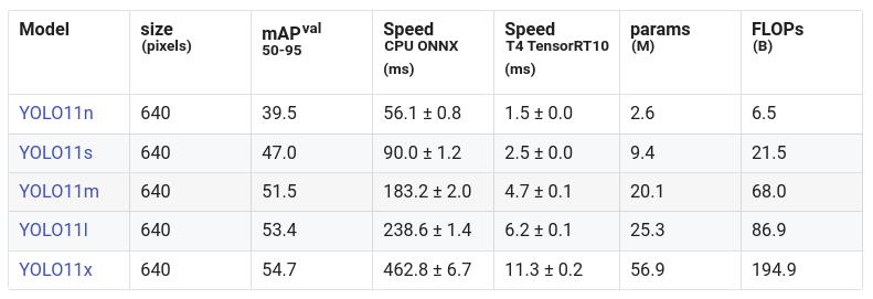
YOLO11 is the latest iteration of the YOLO series from Ultralytics. YOLO11 comes with super lightweight models that are much faster and more efficient than the previous YOLOs. YOLO11 is capable of doing a wider range of computer vision tasks. Ultralytics released five YOLO11 models according to the size and 25 models across all tasks:
- YOLO11n – Nano for small and lightweight tasks.
- YOLO11s – Small upgrade of Nano with some extra accuracy.
- YOLO11m – Medium for general-purpose use.
- YOLO11l – Large for higher accuracy with higher computation.
- YOLO11x – Extra-large for maximum accuracy and performance.
YOLO11 is built on top of the Ultralytics YOLOv8 codebase with some architectural modifications. It also integrates new features (refining those features) from previous YOLOs (like YOLOv9 and YOLOv10) for improved performance. We will explore the new changes in the architecture and codebase later in the blog post. But before we start with YOLO11, let’s recap about YOLO and its architectural improvements over the years. It will help catch up with the concepts faster here.
YOLO Master Post – Every Model Explained
Don’t miss out on this comprehensive resource, Mastering All Yolo Models, for a richer, more informed perspective on the YOLO series.
Applications of YOLO11
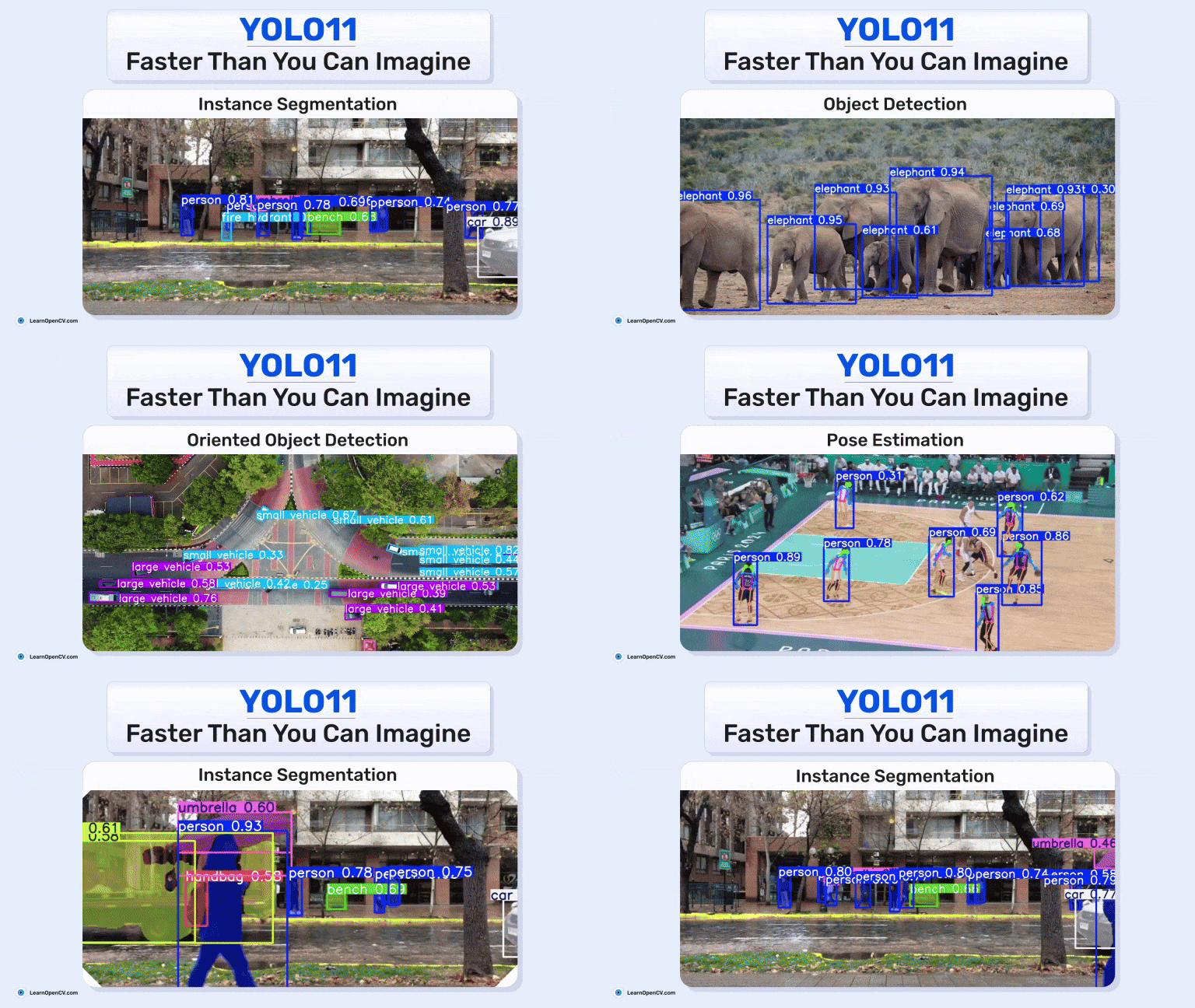
YOLO is mostly known for its object-detection models. However, YOLO11 can do multiple computer vision tasks, like YOLOv8. It includes:
- Object Detection
- Instance Segmentation
- Image Classification
- Pose Estimation
- Oriented Object Detection (OBB)
Let’s explore all of them.
Object Detection
YOLO11 performs object detection by passing the input image into a CNN to extract features. Then, the network predicts bounding boxes and class probabilities for objects within these grids. To handle multi-scale detection, layers are used to ensure objects of various sizes are detected. These predictions are then refined using non-maximum suppression (NMS) to filter out duplicate or low-confidence boxes, resulting in more accurate object detection. The YOLO11 is trained on the MS-COCO dataset for object detection, which includes 80 pre-trained classes.
Instance Segmentation
In addition to detecting objects, YOLO11 extends to instance segmentation by adding a mask prediction branch. These models are trained on the MS-COCO dataset, which includes 80 pre-trained classes. This branch generates pixel-wise segmentation masks for each detected object, allowing the model to distinguish between overlapping objects and provide precise outlines of their shapes. The mask branch in the head processes feature maps and outputs the object masks, enabling pixel-level accuracy in recognizing and differentiating objects within the image.
Pose Estimation
YOLO11 performs pose estimation by detecting and predicting key points on the object, such as joints in a human body. The key points are connected to form the skeleton structure, which represents the pose. These models are trained on COCO, which includes one pre-trained class, ‘person.’
Pose estimation layers are added in the head, and the network is trained to predict the coordinates of key points. A post-processing step connects the points to form the skeleton structure, enabling real-time pose recognition.
Image Classification
For image classification, YOLO11 uses its deep neural network to extract high-level features from an input image and assign it to one of several predefined categories. These models are trained on ImageNet, which includes 1000 pre-trained classes. The network processes the image through multiple layers of convolutions and pooling, reducing spatial dimensions while enhancing essential features. A classification head at the top of the network outputs the predicted class, making it suitable for tasks where identifying the overall category of an image is required.
Oriented Object Detection (OBB)
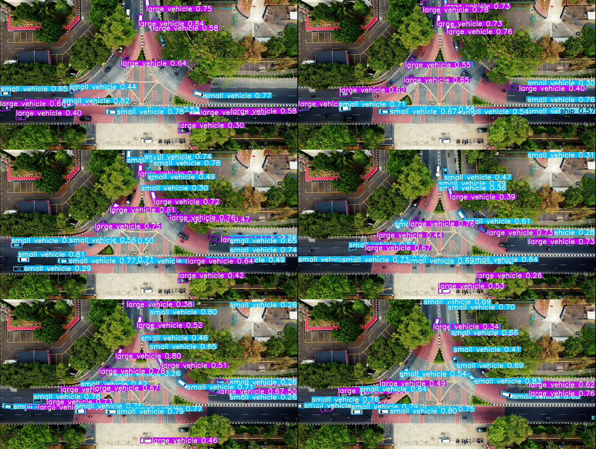
YOLO11 extends regular object detection by incorporating OBB, which allows the model to detect and classify objects that are rotated or have an irregular orientation. This is particularly useful for applications such as aerial image analysis. These models are trained on DOTAv1, which includes 15 pre-trained classes.
The OBB model outputs not only the bounding box coordinates but also the angle of rotation (θ) or the four corner points. These coordinates are used to create bounding boxes that align with the object’s orientation, improving detection accuracy for rotated objects.
YOLO11 Architecture and What’s New in YOLO11?
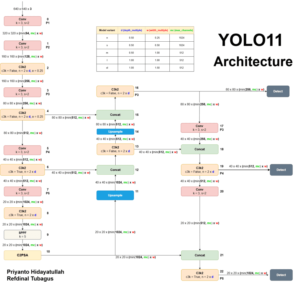
YOLO11 Architecture is an upgrade over YOLOv8 architecture with some new integrations and parameter tuning. Before we proceed to the main part, you can check out our detailed article on YOLOv8 to get an overview of the architecture. Now, if you look at the config file of YOLO11:
# Parameters
nc: 80 # number of classes
scales: # model compound scaling constants, i.e. 'model=yolo11n.yaml' will call yolo11.yaml with scale 'n'
# [depth, width, max_channels]
n: [0.50, 0.25, 1024] # summary: 319 layers, 2624080 parameters, 2624064 gradients, 6.6 GFLOPs
s: [0.50, 0.50, 1024] # summary: 319 layers, 9458752 parameters, 9458736 gradients, 21.7 GFLOPs
m: [0.50, 1.00, 512] # summary: 409 layers, 20114688 parameters, 20114672 gradients, 68.5 GFLOPs
l: [1.00, 1.00, 512] # summary: 631 layers, 25372160 parameters, 25372144 gradients, 87.6 GFLOPs
x: [1.00, 1.50, 512] # summary: 631 layers, 56966176 parameters, 56966160 gradients, 196.0 GFLOPs
# YOLO11n backbone
backbone:
# [from, repeats, module, args]
- [-1, 1, Conv, [64, 3, 2]] # 0-P1/2
- [-1, 1, Conv, [128, 3, 2]] # 1-P2/4
- [-1, 2, C3k2, [256, False, 0.25]]
- [-1, 1, Conv, [256, 3, 2]] # 3-P3/8
- [-1, 2, C3k2, [512, False, 0.25]]
- [-1, 1, Conv, [512, 3, 2]] # 5-P4/16
- [-1, 2, C3k2, [512, True]]
- [-1, 1, Conv, [1024, 3, 2]] # 7-P5/32
- [-1, 2, C3k2, [1024, True]]
- [-1, 1, SPPF, [1024, 5]] # 9
- [-1, 2, C2PSA, [1024]] # 10
# YOLO11n head
head:
- [-1, 1, nn.Upsample, [None, 2, "nearest"]]
- [[-1, 6], 1, Concat, [1]] # cat backbone P4
- [-1, 2, C3k2, [512, False]] # 13
- [-1, 1, nn.Upsample, [None, 2, "nearest"]]
- [[-1, 4], 1, Concat, [1]] # cat backbone P3
- [-1, 2, C3k2, [256, False]] # 16 (P3/8-small)
- [-1, 1, Conv, [256, 3, 2]]
- [[-1, 13], 1, Concat, [1]] # cat head P4
- [-1, 2, C3k2, [512, False]] # 19 (P4/16-medium)
- [-1, 1, Conv, [512, 3, 2]]
- [[-1, 10], 1, Concat, [1]] # cat head P5
- [-1, 2, C3k2, [1024, True]] # 22 (P5/32-large)
- [[16, 19, 22], 1, Detect, [nc]] # Detect(P3, P4, P5)
The changes on the architecture level:
1. Backbone
The backbone is the part of the model that extracts features from the input image at multiple scales. It typically involves stacking convolutional layers and blocks to create feature maps at different resolutions.
Conv Layers: YOLO11 has a similar structure with initial convolution layers to downsample the image:
- [-1, 1, Conv, [64, 3, 2]] # 0-P1/2
- [-1, 1, Conv, [128, 3, 2]] # 1-P2/4
- C3k2 Block: Instead of C2f, YOLO11 introduces the C3k2 block, which is more efficient in terms of computation. This block is a custom implementation of the CSP Bottleneck, which uses two convolutions instead of one large convolution (as in YOLOv8).
- CSP (Cross Stage Partial): CSP networks split the feature map and process one part through a bottleneck layer while merging the other part with the output of the bottleneck. This reduces the computational load and improves feature representation.
- [-1, 2, C3k2, [256, False, 0.25]]
- The C3k2 block also uses a smaller kernel size (indicated by the k2), making it faster while retaining performance.
SPPF and C2PSA: YOLO11 retains the SPPF block but adds a new C2PSA block after SPPF:
- [-1, 1, SPPF, [1024, 5]]
- [-1, 2, C2PSA, [1024]
- The C2PSA (Cross Stage Partial with Spatial Attention) block enhances the spatial attention in the feature maps, improving the model’s focus on the important parts of the image. This gives the model the ability to focus on specific regions of interest more effectively by pooling features spatially.
2. Neck
The neck is responsible for aggregating features from different resolutions and passing them to the head for prediction. It typically involves upsampling and concatenation of feature maps from different levels.
C3k2 Block: YOLO11 replaces the C2f block in the neck with the C3k2 block. As discussed earlier, C3k2 is a faster and more efficient block. For example, after upsampling and concatenation, the neck in YOLO11 looks like this:
- [-1, 2, C3k2, [512, False]] # P4/16-medium
- This change improves the speed and performance of the feature aggregation process.
- Attention Mechanism: YOLO11 focuses more on spatial attention through C2PSA, which helps the model to focus on the key regions in the image for better detection. This is missing in YOLOv8, making YOLO11 potentially more accurate in detecting smaller or occluded objects.
3. Head
The head is the part of the model responsible for generating the final predictions. In object detection, this usually means generating bounding boxes and classifying the objects inside those boxes.
C3k2 Block: Similar to the neck, YOLO11 replaces the C2f block in the head.
- [-1, 2, C3k2, [512, False]] # P4/16-medium
Detect Layer: The final Detect layer is the same as in YOLOv8:
- [[16, 19, 22], 1, Detect, [nc]] # Detect(P3, P4, P5)
The use of C3k2 blocks makes the model faster in terms of inference and more efficient in terms of parameters.
So, Let’s see how the new blocks (layers) look in the code:
C3k2 Block (from blocks.py):
C3k2 is a faster and more efficient variant of the CSP bottleneck. It uses two convolutions instead of one large convolution, which speeds up feature extraction.
class C3k2(C2f):
def __init__(self, c1, c2, n=1, c3k=False, e=0.5, g=1, shortcut=True):
super().__init__(c1, c2, n, shortcut, g, e)
self.m = nn.ModuleList(
C3k(self.c, self.c, 2, shortcut, g) if c3k else Bottleneck(self.c, self.c, shortcut, g) for _ in range(n)
)
C3k Block (from blocks.py):
C3k is a more flexible bottleneck module that allows for customizable kernel sizes. This is useful for extracting more detailed features in images.
class C3k(C3):
def __init__(self, c1, c2, n=1, shortcut=True, g=1, e=0.5, k=3):
super().__init__(c1, c2, n, shortcut, g, e)
c_ = int(c2 * e) # hidden channels
self.m = nn.Sequential(*(Bottleneck(c_, c_, shortcut, g, k=(k, k), e=1.0) for _ in range(n)))
C2PSA Block (from blocks.py):
C2PSA (Cross Stage Partial with Spatial Attention) enhances the model’s spatial attention capability. This block adds attention to the feature maps, helping the model focus on important regions of the image.
class C2PSA(nn.Module):
def __init__(self, c1, c2, e=0.5):
super().__init__()
c_ = int(c2 * e)
self.cv1 = Conv(c1, c_, 1, 1)
self.cv2 = Conv(c1, c_, 1, 1)
self.cv3 = Conv(2 * c_, c2, 1)
def forward(self, x):
return self.cv3(torch.cat((self.cv1(x), self.cv2(x)), 1))
The Ultralytics team has not released an architecture diagram yet, but they plan to do so in the future. We will update the diagram here; you can keep your eye on this GitHub thread for updates.
YOLO11 Code Pipeline
Now we have an idea about the architecture. So, let’s see how the codebase is structured:
In the ultralytics GitHub repo, we will mainly focus on,
- Modules in nn/modules/
- block.py
- conv.py
- head.py
- transformer.py
- utils.py
- The nn/tasks.py File
Overview of the Codebase
The codebase is structured into modules that define various neural network components used in the YOLO11 model. These components are organized into different files within the nn/modules/ directory:
- block.py: Defines various building blocks (modules) used in the model, such as bottlenecks, CSP modules, and attention mechanisms.
- conv.py: Contains convolutional modules, including standard convolutions, depth-wise convolutions, and other variations.
- head.py: Implements the head of the model responsible for producing the final predictions (e.g., bounding boxes, class probabilities).
- transformer.py: Includes transformer-based modules, which are used for attention mechanisms and advanced feature extraction.
- utils.py: Provides utility functions and helper classes used across the modules.
- The nn/tasks.py file defines the different task-specific models (e.g., detection, segmentation, classification) that combine these modules to form complete architectures.
Modules in nn/modules/
As discussed previously, YOLO11 is built on top of the YOLOv8 codebase. So, we will mainly focus on the updated scripts: block.py, conv.py, and head.py here.
block.py
This file defines various building blocks used in the YOLO11 model. These blocks are essential components that form the layers of the neural network.
Key Components:
Bottleneck Modules:
- Bottleneck: A standard bottleneck module with optional shortcut connections.
- Res: A residual block that uses a series of convolutions and an identity shortcut.
class Bottleneck(nn.Module):
def __init__(self, c1, c2, shortcut=True, g=1, e=0.5):
super().__init__()
c_ = int(c2 * e)
self.cv1 = Conv(c1, c_, 1, 1)
self.cv2 = Conv(c_, c2, 3, 1, g=g)
self.add = shortcut and c1 == c2
def forward(self, x):
return x + self.cv2(self.cv1(x)) if self.add else self.cv2(self.cv1(x))
- The Bottleneck class implements a bottleneck module, which reduces the number of channels (dimensionality reduction) and then expands them again.
- Components:
- self.cv1: A 1×1 convolution that reduces the number of channels.
- self.cv2: A 3×3 convolution that increases the number of channels back to the original.
- self.add: A boolean indicating whether to add a shortcut connection.
- Forward Pass: The input x is passed through cv1 and cv2. If self.add is True, the original input x is added to the output (residual connection).
CSP (Cross Stage Partial) Modules:
- BottleneckCSP: A CSP version of the bottleneck module.
- CSPBlock: A more complex CSP module with multiple bottleneck layers.
class BottleneckCSP(nn.Module):
def __init__(self, c1, c2, n=1, shortcut=True, g=1, e=0.5):
super().__init__()
c_ = int(c2 * e)
self.cv1 = Conv(c1, c_, 1, 1)
self.cv2 = nn.Sequential(
*[Bottleneck(c_, c_, shortcut, g, e=1.0) for _ in range(n)]
)
self.cv3 = Conv(2 * c_, c2, 1)
self.add = c1 == c2
def forward(self, x):
y1 = self.cv2(self.cv1(x))
y2 = x if self.add else None
return self.cv3(torch.cat((y1, y2), 1)) if y2 is not None else self.cv3(y1)
- The CSPBottleneck module divides the feature map into two parts. One part goes through a series of bottleneck layers, and the other part is connected directly to the output, reducing computational cost and enhancing gradient flow.
- Components:
- self.cv1: Reduces the number of channels.
- self.cv2: A sequence of bottleneck layers.
- self.cv3: Combines the features and adjusts the number of channels.
- self.add: Determines if a shortcut connection is added.
Other Modules:
- SPPF: Spatial Pyramid Pooling Fast module, which performs pooling at multiple scales.
- Concat: Concatenates multiple tensors along a specified dimension.
class SPPF(nn.Module):
def __init__(self, c1, c2, k=5):
super().__init__()
c_ = c1 // 2
self.cv1 = Conv(c1, c_, 1, 1)
self.cv2 = Conv(c_ * 4, c2, 1, 1)
self.m = nn.MaxPool2d(kernel_size=k, stride=1, padding=k // 2)
def forward(self, x):
x = self.cv1(x)
y1 = self.m(x)
y2 = self.m(y1)
y3 = self.m(y2)
return self.cv2(torch.cat([x, y1, y2, y3], 1))
- The SPPF module performs max pooling at different scales and concatenates the results to capture features at multiple spatial scales.
- Components:
- self.cv1: Reduces the number of channels.
- self.cv2: Adjusts the number of channels after concatenation.
- self.m: Max pooling layer.
- Forward Pass: The input x is passed through cv1, then through three consecutive max pooling layers (y1, y2, y3). The results are concatenated and passed through cv2.
conv.py
This file contains various convolutional modules, including standard and specialized convolutions.
Key Components:
Standard Convolution Module (Conv):
class Conv(nn.Module):
default_act = nn.SiLU() # default activation
def __init__(self, c1, c2, k=1, s=1, p=None, g=1, d=1, act=True):
super().__init__()
self.conv = nn.Conv2d(c1, c2, k, s, autopad(k, p, d), groups=g, dilation=d, bias=False)
self.bn = nn.BatchNorm2d(c2)
self.act = self.default_act if act is True else act if isinstance(act, nn.Module) else nn.Identity()
def forward(self, x):
return self.act(self.bn(self.conv(x)))
- Implements a standard convolutional layer with batch normalization and activation.
- Components:
- self.conv: The convolutional layer.
- self.bn: Batch normalization.
- self.act: Activation function (default is nn.SiLU()).
- Forward Pass: Applies convolution, followed by batch normalization and activation.
Depth-wise Convolution (DWConv):
class DWConv(Conv):
def __init__(self, c1, c2, k=1, s=1, d=1, act=True):
super().__init__(c1, c2, k, s, g=math.gcd(c1, c2), d=d, act=act)
- Performs depth-wise convolution, where each input channel is convolved separately.
- Components:
- Inherits from Conv.
- Sets groups parameter to the greatest common divisor of c1 and c2, effectively grouping the convolution per channel.
Other Convolutional Modules:
- Conv2: Simplified version of RepConv, which is used for model compression and acceleration.
- GhostConv: Implements GhostNet’s ghost module, which reduces redundancy in feature maps.
- RepConv: Re-parameterizable convolutional layer that can be converted from training to inference mode.
head.py
This file implements the head modules responsible for producing the final predictions of the model.
Key Components:
Detection Head (Detect):
class Detect(nn.Module):
def __init__(self, nc=80, ch=()):
super().__init__()
self.nc = nc # number of classes
self.nl = len(ch) # number of detection layers
self.reg_max = 16 # DFL channels
self.no = nc + self.reg_max * 4 # number of outputs per anchor
self.stride = torch.zeros(self.nl) # strides computed during build
# Define layers
self.cv2 = nn.ModuleList(
nn.Sequential(Conv(x, c2, 3), Conv(c2, c2, 3), nn.Conv2d(c2, 4 * self.reg_max, 1)) for x in ch
)
self.cv3 = nn.ModuleList(
nn.Sequential(
nn.Sequential(DWConv(x, x, 3), Conv(x, c3, 1)),
nn.Sequential(DWConv(c3, c3, 3), Conv(c3, c3, 1)),
nn.Conv2d(c3, self.nc, 1),
)
for x in ch
)
self.dfl = DFL(self.reg_max) if self.reg_max > 1 else nn.Identity()
- The Detect class defines the detection head that outputs bounding box coordinates and class probabilities.
- Components:
- self.cv2: Convolutional layers for bounding box regression.
- self.cv3: Convolutional layers for classification.
- self.dfl: Distribution Focal Loss module for bounding box refinement.
- Forward Pass: Processes the input feature maps and outputs predictions for bounding boxes and classes.
Segmentation Head (Segment):
class Segment(Detect):
def __init__(self, nc=80, nm=32, npr=256, ch=()):
super().__init__(nc, ch)
self.nm = nm # number of masks
self.npr = npr # number of prototypes
self.proto = Proto(ch[0], self.npr, self.nm) # protos
c4 = max(ch[0] // 4, self.nm)
self.cv4 = nn.ModuleList(nn.Sequential(Conv(x, c4, 3), Conv(c4, c4, 3), nn.Conv2d(c4, self.nm, 1)) for x in ch)
- Extends the Detect class to include segmentation capabilities.
- Components:
- self.proto: Generates mask prototypes.
- self.cv4: Convolutional layers for mask coefficients.
- Forward Pass: Outputs bounding boxes, class probabilities, and mask coefficients.
Pose Estimation Head (Pose):
class Pose(Detect):
def __init__(self, nc=80, kpt_shape=(17, 3), ch=()):
super().__init__(nc, ch)
self.kpt_shape = kpt_shape # number of keypoints, number of dimensions
self.nk = kpt_shape[0] * kpt_shape[1] # total number of keypoint outputs
c4 = max(ch[0] // 4, self.nk)
self.cv4 = nn.ModuleList(nn.Sequential(Conv(x, c4, 3), Conv(c4, c4, 3), nn.Conv2d(c4, self.nk, 1)) for x in ch)
- Extends the Detect class for human pose estimation tasks.
- Components:
- self.kpt_shape: Shape of the keypoints (number of keypoints, dimensions per keypoint).
- self.cv4: Convolutional layers for keypoint regression.
- Forward Pass: Outputs bounding boxes, class probabilities, and keypoint coordinates.
3. The nn/tasks.py
nn/tasks.py
is the parent code to execute all the YOLO11 models to do the compute vision tasks, including detection, segmentation, pose estimation, and classification models.
# This is a summarized version of the original script
class BaseModel(nn.Module):
# Base model class for YOLOv8 models
def forward(self, x, *args, **kwargs):
# Forward pass: handles both training (loss) and inference (predict)
if isinstance(x, dict):
return self.loss(x, *args, **kwargs) # Training: loss
return self.predict(x, *args, **kwargs) # Inference: prediction
class DetectionModel(BaseModel):
# YOLOv8 detection model class
def __init__(self, cfg="yolov8n.yaml", ch=3, nc=None, verbose=True):
super().__init__()
# Model setup (config parsing, layers, etc.)
self.yaml = cfg if isinstance(cfg, dict) else yaml_model_load(cfg)
self.model, self.save = parse_model(deepcopy(self.yaml), ch=ch, verbose=verbose)
# Stride and bias initialization (omitted details for brevity)
m = self.model[-1]
if isinstance(m, Detect):
s = 256
m.stride = torch.tensor([s / x.shape[-2] for x in self._predict_once(torch.zeros(1, ch, s, s))])
self.stride = m.stride
m.bias_init()
class SegmentationModel(DetectionModel):
# YOLOv8 segmentation model class
def __init__(self, cfg="yolov8n-seg.yaml", ch=3, nc=None, verbose=True):
super().__init__(cfg=cfg, ch=ch, nc=nc, verbose=verbose)
def init_criterion(self):
# Return the segmentation-specific loss function
return v8SegmentationLoss(self)
class PoseModel(DetectionModel):
# YOLOv8 pose estimation model class
def __init__(self, cfg="yolov8n-pose.yaml", ch=3, nc=None, data_kpt_shape=(None, None), verbose=True):
if not isinstance(cfg, dict):
cfg = yaml_model_load(cfg)
if list(data_kpt_shape) != list(cfg["kpt_shape"]):
cfg["kpt_shape"] = data_kpt_shape
super().__init__(cfg=cfg, ch=ch, nc=nc, verbose=verbose)
def init_criterion(self):
# Return the pose-specific loss function
return v8PoseLoss(self)
class ClassificationModel(BaseModel):
# YOLOv8 classification model class
def __init__(self, cfg="yolov8n-cls.yaml", ch=3, nc=None, verbose=True):
super().__init__()
self._from_yaml(cfg, ch, nc, verbose)
def _from_yaml(self, cfg, ch, nc, verbose):
# Parse config and set up model layers
self.yaml = cfg if isinstance(cfg, dict) else yaml_model_load(cfg)
self.model, self.save = parse_model(deepcopy(self.yaml), ch=ch, verbose=verbose)
self.names = {i: f"{i}" for i in range(self.yaml["nc"])}
class Ensemble(nn.ModuleList):
# Ensemble class to combine multiple models' outputs
def __init__(self):
super().__init__()
def forward(self, x, augment=False, profile=False, visualize=False):
# Forward pass for ensemble, combining outputs from all models
y = [module(x, augment, profile, visualize)[0] for module in self]
return torch.cat(y, 2), None
It starts with defining the BaseModel
class, which serves as a foundation for all the models, with the forward
method handling both training (via the loss
function) and inference (via the predict
function).
The DetectionModel
class extends BaseModel
and specializes in object detection, implementing stride initialization and layer fusion for efficiency using the fuse
method.
The SegmentationModel
and PoseModel
further, extend DetectionModel
, adding functionality specific to segmentation and pose estimation tasks, and each initializes its loss functions like v8SegmentationLoss
and v8PoseLoss
.
The ClassificationModel
handles classification tasks and reshapes the output layer based on the number of classes (nc
). Additionally, the Ensemble
class is included to combine outputs from multiple models. Helper functions such as parse_model, yaml_model_load, and fuse_conv_and_bn are used for model parsing, configuration loading, and inference layer optimization.
Download the Code Here
YOLO11 Inference
Now, it’s time to do some experiments with YOLO11 models and see the inference results. We have taken a Video by Usha Jey titled Hybrid Bharatham to run the inference. Now, we will explore object detection, instance segmentation, and pose estimation tasks one by one:
We are using Nvidia Geforce RTX 3070 Ti Laptop GPU to run the inference. Let’s start:
First, we need to set up our environment:
We’ll use the pre-trained weights of YOLO11 from the Ultralytics GitHub for our inference experiments. To do the inference, you need to clone the Ultralytics repository by the following command:
! git clone https://github.com/ultralytics/ultralytics.git
! cd ultralytics
Then, we need to set up the environment using the following command:
! conda create -n yolo11 python=3.11
! conda activate yolo11
! pip install ultralytics
We are using miniconda to create the virtual environment. Within the environment, we need to install the Ultralytics Python package.
Object Detection
For object detection, we will run this command:
! yolo detect predict model=yolo11x.pt source='./path/to/your/video.mp4' save=True classes=[0]
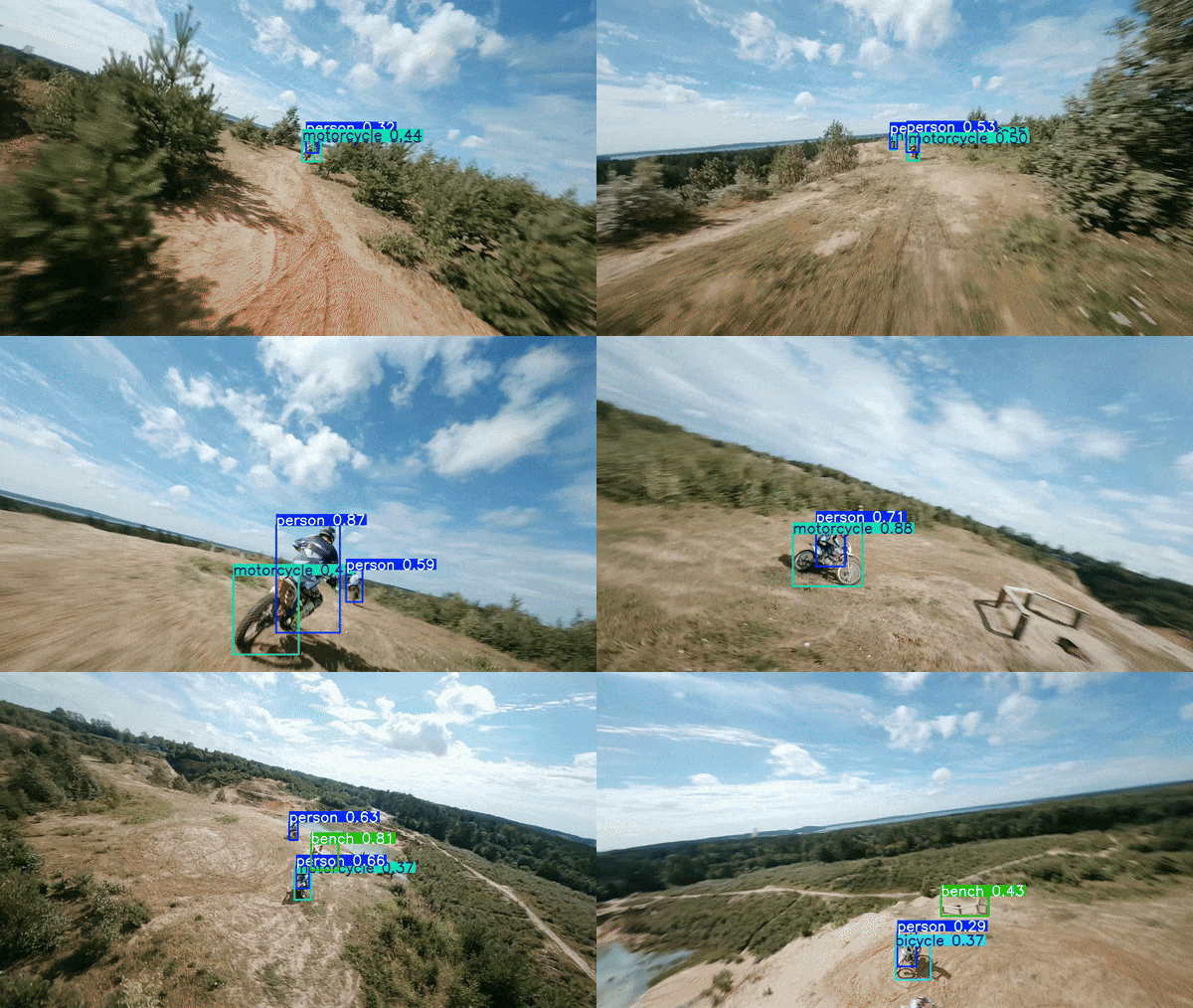
Here, for this video, we know there are only persons in the frame, so we have just filtered out the person class detections. You can fine-tune all the other inference arguments that are available. Visit ultralytics documentation for more info.
This is the result that we get:
Instance Segmentation
For instance segmentation, run this command:
! yolo segment predict model=yolo11x.pt source='./path/to /your/video.mp4' save=True classes=[0]
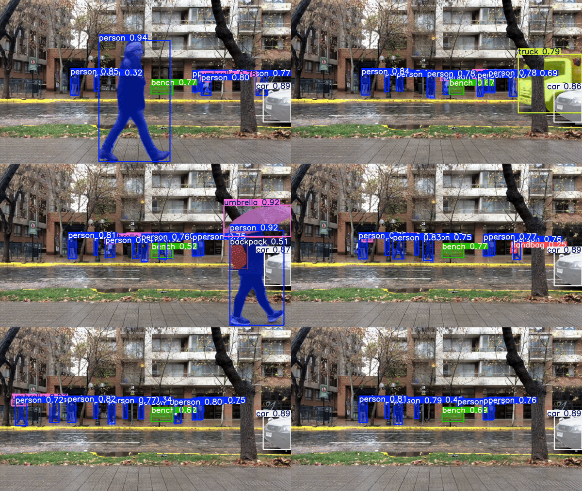
And the result:
Pose Estimation
For pose estimation, run:
! yolo pose predict model=yolo11x-pose.pt source='./path/to/your/video.mp4' save=True classes=[0]
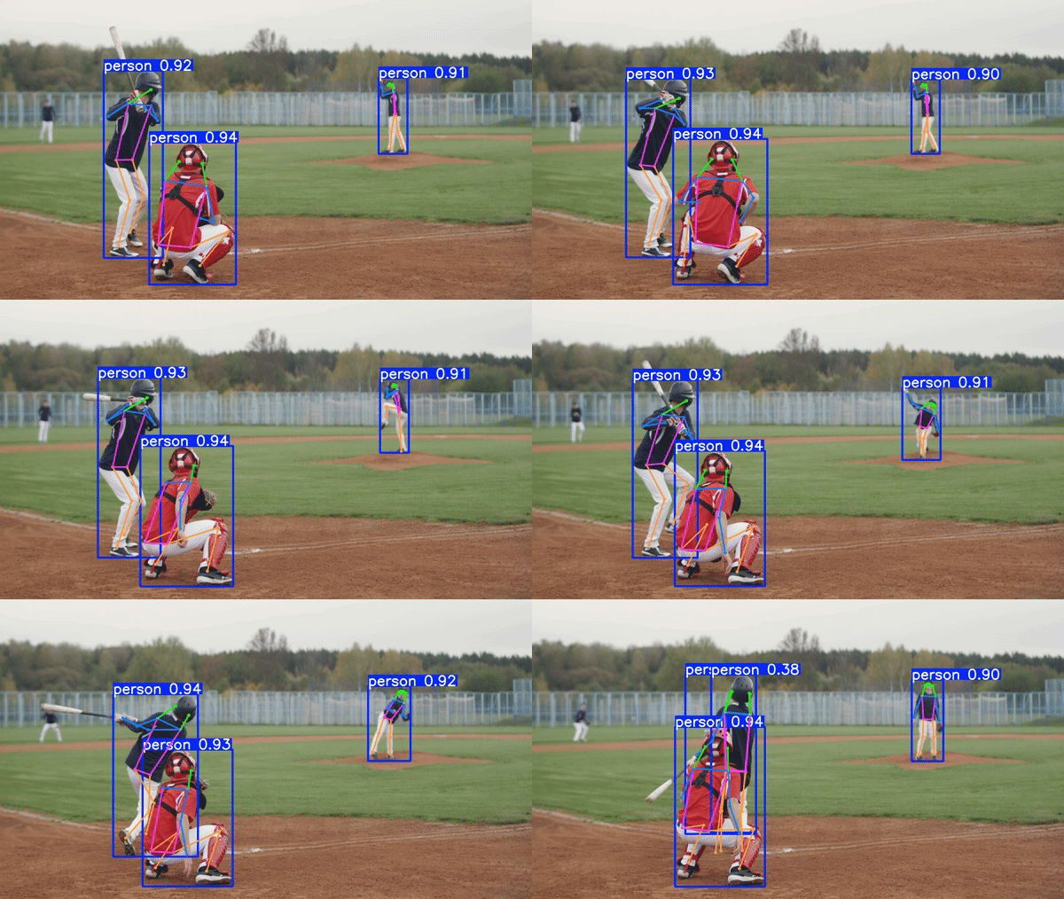
The inference result:
Using just one YOLO11 model, you can analyze every aspect of your input video. Isn’t that amazing?
Oriented Object Detection (OBB)
But wait, it’s not the end. We know YOLO11 can detect small objects as well. Let’s try that out, too:
For that, we need to run the command:
! yolo obb predict model=yolo11x-obb.pt source='./path/to/your/video.mp4' save=True
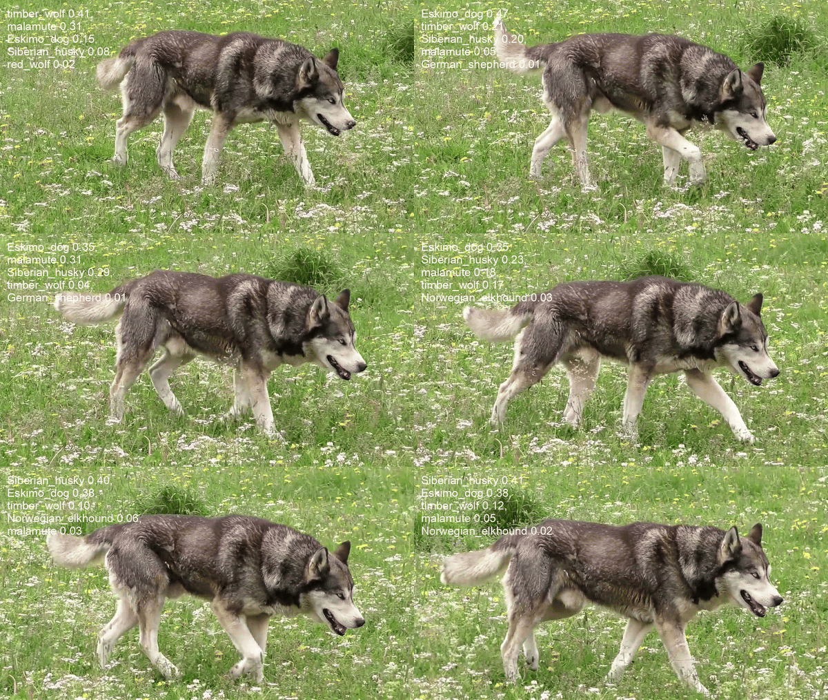
Here is the result:
YOLO11 vs YOLOv10
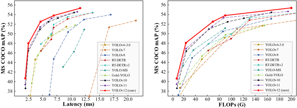
From the plot, it seems that YOLO11l and YOLO11x are slower than YOLOv10, and YOLO11n is the same as YOLOv10n. So, why not clear up the controversy by doing a hands-on comparison with both models?
So, we will compare YOLO11 with the last released YOLOv10 and see the performance benchmarks for both models. We ran all the inferences on the Nvidia Geforce RTX 3070 Ti Laptop GPU.
First, we will compare YOLOv10n (2.3M Params) with YOLO11n (2.6M params) model. We ran inference on the same video and compared the latency and FPS The benchmarks for you:
YOLOv11n
Speed: 1.4ms preprocess, 3.9ms inference, 1.2ms postprocess per image at shape (1, 3, 384, 640)
FPS(inference): 256
YOLOv10n
Speed: 1.4ms preprocess, 4.5ms inference, 0.4ms postprocess per image at shape (1, 3, 384, 640)
FPS(inference): 222
Now, we will compare YOLOv10x (29.5M Params) with YOLO11x (56.9M Params). We ran inference on the same video and compared the latency and FPS. Benchmarks we got:
YOLOv11x
Speed: 1.4ms preprocess, 18.5ms inference, 1.6ms postprocess per image at shape (1, 3, 384, 640)
FPS(inference): 54
YOLOv10x
Speed: 1.4ms preprocess, 16.8ms inference, 0.6ms postprocess per image at shape (1, 3, 384, 640)
FPS(inference): 59
As you can see for the Nano models, YOLO11 performed better even with a higher param size. Also, like YOLOv10, the Ultralytics team plans to fully e2e models soon. You can keep your eye on this thread.
Quick Recap
- Lightweight and Efficient: The YOLO11 is the lightest and fastest model in the YOLO family. It features five different sizes (Nano, Small, Medium, Large, and Extra-large) to suit various use cases, from lightweight tasks to high-performance applications.
- New Architectures: YOLO11 introduces new architectural improvements like the C3k2 block, SPPF, and C2PSA, making the model more efficient in extracting and processing features and improving attention on key areas of an image.
- Multi-Task Capabilities: In addition to object detection, YOLO11 can handle instance segmentation, image classification, pose estimation, and oriented object detection (OBB), making it highly versatile in computer vision tasks.
- Enhanced Attention Mechanisms: The integration of spatial attention mechanisms like C2PSA in the architecture helps YOLO11 focus more effectively on essential regions in the image, improving its detection accuracy, particularly for complex or occluded objects.
- Benchmark Superiority: In direct comparison to YOLOv10, YOLO11 shows superior performance, particularly in the Nano model series. Despite having more parameters, YOLO11n outperforms YOLOv10n in terms of inference speed and FPS, making it a highly efficient model for real-time applications without sacrificing accuracy or computational efficiency.
Conclusion
We have explored YOLO11 and its capabilities so far. We hope you have a good understanding of the model architecture and code pipeline. Build cool projects with YOLO11, and make sure to share them with us! See you in the next one.
This article has been promoted by Ultralytics, which made it the official article of YOLO11.
References
Ultralytics YOLO11 Overview Article