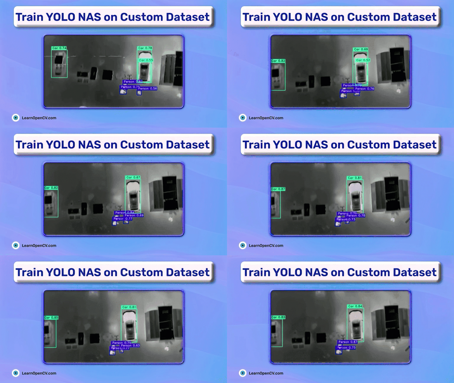
YOLO-NAS is currently the latest YOLO object detection model. From the outset, it beats all other YOLO models in terms of accuracy. The pretrained YOLO-NAS models detect more objects with better accuracy compared to the previous YOLO models. But how do we train YOLO NAS on a custom dataset? This will be our goal in this article – to train different YOLO NAS models on a custom dataset.
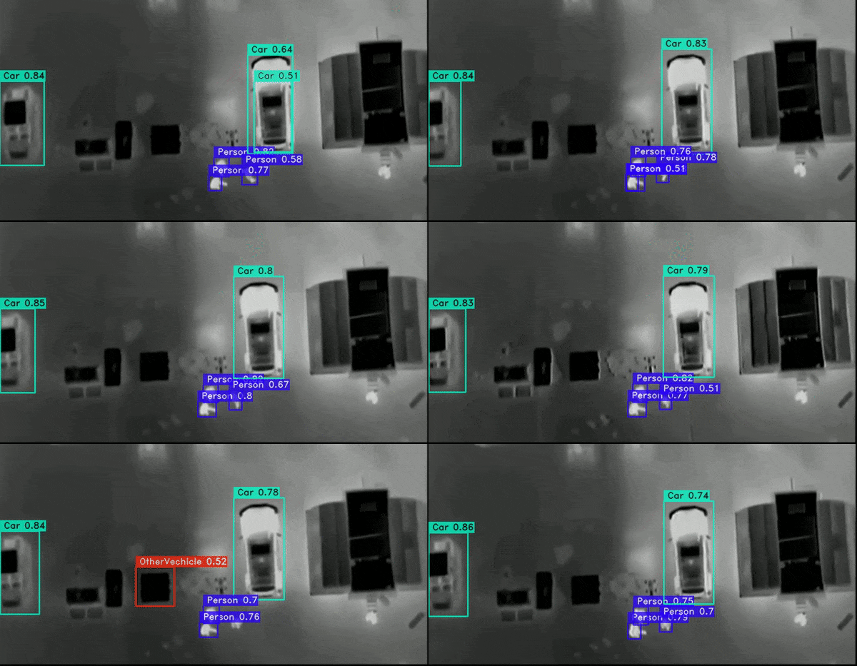
The primary claim of YOLO-NAS is that it can detect smaller objects better than the previous models. Although we can run several inference experiments to analyze the results, training it on a challenging dataset will give us a better understanding. To this effect, we will run four training experiments using the three available pretrained YOLO-NAS models. For this purpose, we choose a UAV thermal imaging detection dataset.
During the experimentation process, we will traverse the complete training pipeline for YOLO-NAS.
- The Object Detection Dataset to Train YOLO NAS
- Train YOLO NAS on Custom Dataset
- Fine Tuning YOLO NAS Models
- Inference on Test Images using the Trained YOLO NAS Model
- YOLO NAS Trained Model Video Inference Results
- Conclusion
YOLO Master Post – Every Model Explained
Don’t miss out on this comprehensive resource, Mastering All Yolo Models for a richer, more informed perspective on the YOLO series.
The Object Detection Dataset to Train YOLO NAS
Let’s start by getting familiar with the UAV High-altitude Infrared Thermal Dataset.
It contains thermal drone imagery during nighttime. Given the high-altitude recording from the drone, most of the objects appear small. This makes the dataset a difficult one to solve for most object detection models. However, it makes the perfect custom dataset to train YOLO-NAS to check its accuracy on small objects.
The dataset contains 2898 thermal images across 5 object classes:
- Person
- Car
- Bicycle
- OtherVehicle
- DontCare
The dataset already contains train, validation, and test splits. There are 2008 training, 287 validation, and 571 test samples. The dataset is already present in YOLO annotation format.
The following are some of the unannotated ground truth images from the dataset.
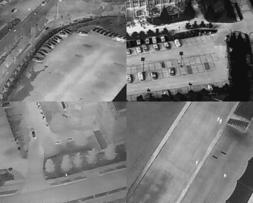
It is very clear that apart from cars, the human eye cannot see the other objects on the ground without proper annotation.
To get a perspective of where each object is, have a look at some of the annotated images.
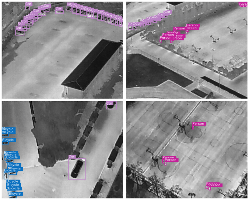
The above figure helps to get a better understanding of the dataset objects. This also tells us how difficult it is for the human eyes to detect objects like persons and bicycles in this dataset. Hopefully, the YOLO-NAS model will do a much better job than us humans after training.
Train YOLO NAS on Custom Dataset
Moving forward, we will delve into the coding part of this article. Upon downloading the code for this article, you will discover three notebooks.
YOLO_NAS_Fine_Tuning.ipynbYOLO_NAS_Large_Fine_Tuning.ipynbinference.ipynb
We will go through the YOLO_NAS_Fine_Tuning.ipynb notebooks in considerable detail. These two contain all the steps you need to train YOLO NAS on the custom dataset and run inference using the trained models later on. The training notebooks contain the code to download the dataset.
The code that follows will train three YOLO NAS models:
- YOLO NAS s (Small)
- YOLO NAS m (Medium)
- YOLO NAS l (Large)
Before getting started, you may install the super-gradients package, which we need throughout the training and inference process. Although the notebooks contain the command to do so, you can also install it using the following command:
pip install super-gradients
Furthermore, if you are interested in the pretrained performance, don’t miss out on the post on YOLO NAS.
Fine Tuning YOLO NAS Models
Let’s dive into the notebook code. The very first step is to import all the necessary packages and modules.
from super_gradients.training import Trainer
from super_gradients.training import dataloaders
from super_gradients.training.dataloaders.dataloaders import (
    coco_detection_yolo_format_train,
    coco_detection_yolo_format_val
)
from super_gradients.training import models
from super_gradients.training.losses import PPYoloELoss
from super_gradients.training.metrics import (
    DetectionMetrics_050,
    DetectionMetrics_050_095
)
from super_gradients.training.models.detection_models.pp_yolo_e import PPYoloEPostPredictionCallback
from tqdm.auto import tqdm

import os
import requests
import zipfile
import cv2
import matplotlib.pyplot as plt
import glob
import numpy as np
import random
Let’s examine all the major imports from the above code block.
Trainer: The Trainer initiates the training process and sets up the experiment directory as well.dataloaders: Super Gradients offers its own dataloaders for hassle-free training of YOLO NAS models.coco_detection_yolo_format_train,coco_detection_yolo_format_val: These two will help us define the training and validation dataset.models: This function will initialize the YOLO NAS models.PPYoloELoss: YOLO NAS uses the PPYoloELoss while training.DetectionMetrics_050,DetectionMetrics_050_095: We will monitor the mAP at 50% IoU and the primary metric while training.
Dataset Download and Directory Structure
The next few code blocks download the dataset and extract it to the current directory, which we will skip here. All the notebooks and datasets are present in the parent dataset directory, whose structure is as below.
hit-uav
├── dataset.yaml
├── images
│   ├── test
│   ├── train
│   └── val
└── labels
    ├── test
    ├── train
    └── val
Dataset Parameters for Training YOLO NAS
The next step involves preparing the dataset in a manner that allows us to run multiple training experiments. First, let’s define all the dataset paths & classes, and also the dataset parameter dictionary.
ROOT_DIR = 'hit-uav'
train_imgs_dir = 'images/train'
train_labels_dir = 'labels/train'
val_imgs_dir = 'images/val'
val_labels_dir = 'labels/val'
test_imgs_dir = 'images/test'
test_labels_dir = 'labels/test'
classes = ['Person', 'Car', 'Bicycle', 'OtherVechicle', 'DontCare']

dataset_params = {
    'data_dir':ROOT_DIR,
    'train_images_dir':train_imgs_dir,
    'train_labels_dir':train_labels_dir,
    'val_images_dir':val_imgs_dir,
    'val_labels_dir':val_labels_dir,
    'test_images_dir':test_imgs_dir,
    'test_labels_dir':test_labels_dir,
    'classes':classes
}
Using the dataset_params we can easily create the datasets in the required format later on. Also, we need to define the number of training epochs, the batch size, and the number of workers for data processing.
# Global parameters.
EPOCHS = 50
BATCH_SIZE = 16
WORKERS = 8
The above hyperparameters and dataset parameters will be used for all three training experiments.
Dataset Preparation for Training YOLO NAS
As we have all the parameters in place, we can define the training and validation datasets.
train_data = coco_detection_yolo_format_train(
    dataset_params={
        'data_dir': dataset_params['data_dir'],
        'images_dir': dataset_params['train_images_dir'],
        'labels_dir': dataset_params['train_labels_dir'],
        'classes': dataset_params['classes']
    },
    dataloader_params={
        'batch_size':BATCH_SIZE,
        'num_workers':WORKERS
    }
)

val_data = coco_detection_yolo_format_val(
    dataset_params={
        'data_dir': dataset_params['data_dir'],
        'images_dir': dataset_params['val_images_dir'],
        'labels_dir': dataset_params['val_labels_dir'],
        'classes': dataset_params['classes']
    },
    dataloader_params={
        'batch_size':BATCH_SIZE,
        'num_workers':WORKERS
    }
)
In the above code block, we create train_data and val_data for training and validation, respectively.
As we can see, we use the dataset_params dictionary to get the dataset path and dataset class values. We also define the dataloader_params for each that accepts the batch size and the number of workers for the data loading process.
You may have noticed that we are excluding the test split at this stage. We are reserving it for later use in order to perform inference with our trained YOLO NAS models.
Defining the Transforms and Augmentations for YOLO NAS Training
Data augmentation is a major part of training any deep learning model. It allows us to train robust models for longer time periods without overfitting. Along the way, the model also learns different features which may not be part of the original dataset.
The data transformation pipeline of Super Gradients offers an effective way to apply and control augmentations.
The following will print all the default transforms being applied to the dataset.
train_data.dataset.transforms
We will see the following output.
[DetectionMosaic('additional_samples_count': 3, 'non_empty_targets': False, 'prob': 1.0, 'input_dim': [640, 640], 'enable_mosaic': True, 'border_value': 114),

 DetectionRandomAffine('additional_samples_count': 0, 'non_empty_targets': False, 'degrees': 10.0,
'translate': 0.1, 'scale': [0.1, 2], 'shear': 2.0, 'target_size': [640, 640], 'enable': True, 'filter_box_candidates': True, 'wh_thr': 2, 'ar_thr': 20, 'area_thr': 0.1, 'border_value': 114),

 DetectionMixup('additional_samples_count': 1, 'non_empty_targets': True, 'input_dim': [640, 640], 'mixup_scale': [0.5, 1.5], 'prob': 1.0, 'enable_mixup': True, 'flip_prob': 0.5, 'border_value': 114),
.
.
.
XYCoordinateFormat object at 0x7efcc5c07340>), ('labels', name=labels length=1)]), 'output_format': OrderedDict([('labels', name=labels length=1), ('bboxes', name=bboxes length=4 format=
<super_gradients.training.datasets.data_formats.bbox_formats.cxcywh.CXCYWHCoordinateFormat object at 0x7efcc5976170>)]), 'max_targets': 120, 'min_bbox_edge_size': 1, 'input_dim': [640, 640], 'targets_format_converter':
<super_gradients.training.datasets.data_formats.format_converter.ConcatenatedTensorFormatConverter object at 0x7efcb956b5b0>)]
Among the many augmentations, one of them is MixUp. However, MixUp can cause the dataset to be extremely difficult to perceive for deep learning models if not handled properly. From initial experiments, we found that MixUp augmentation for this dataset makes the dataset very confusing as it overlaps one image over another. Removing the Mixup augmentation and keeping the others intact seemed to improve the performance.
We can remove the MixUp augmentation from the list by popping the element from index 2.
############ An example on how to modify augmentations ###########
train_data.dataset.transforms.pop(2)
We can also visualize the transformed images using the following code.
train_data.dataset.plot(plot_transformed_data=True)
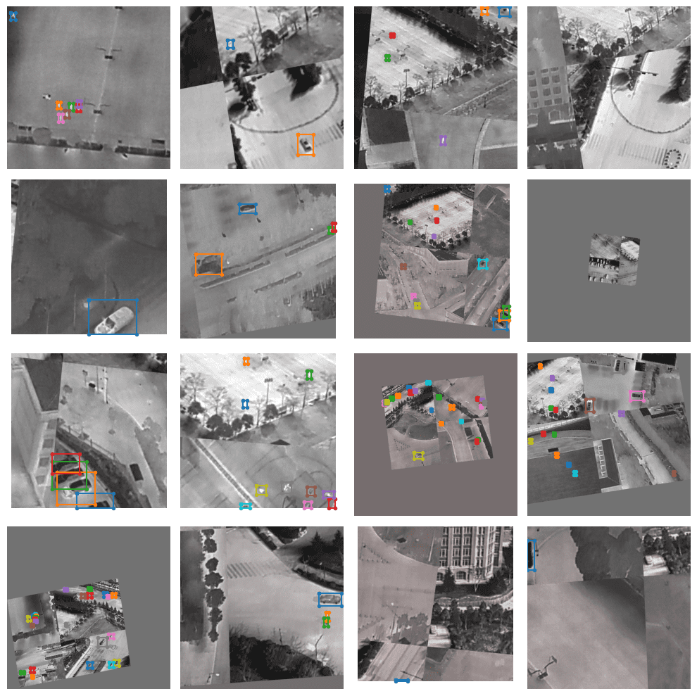
Apart from MixUp, other augmentations like mosaic, rotation, zoom in, and zoom out have also been applied to the images.
The YOLO NAS Training Parameters
The training parameters are the most essential components before we start the fine-tuning process. This is where we define the number of epochs to train, the validation metrics to monitor, and the learning rate, among many others.
train_params = {
    'silent_mode': False,
    "average_best_models":True,
    "warmup_mode": "linear_epoch_step",
    "warmup_initial_lr": 1e-6,
    "lr_warmup_epochs": 3,
    "initial_lr": 5e-4,
    "lr_mode": "cosine",
    "cosine_final_lr_ratio": 0.1,
    "optimizer": "Adam",
    "optimizer_params": {"weight_decay": 0.0001},
    "zero_weight_decay_on_bias_and_bn": True,
    "ema": True,
    "ema_params": {"decay": 0.9, "decay_type": "threshold"},
    "max_epochs": EPOCHS,
    "mixed_precision": True,
    "loss": PPYoloELoss(
        use_static_assigner=False,
        num_classes=len(dataset_params['classes']),
        reg_max=16
    ),
    "valid_metrics_list": [
        DetectionMetrics_050(
            score_thres=0.1,
            top_k_predictions=300,
            num_cls=len(dataset_params['classes']),
            normalize_targets=True,
            post_prediction_callback=PPYoloEPostPredictionCallback(
                score_threshold=0.01,
                nms_top_k=1000,
                max_predictions=300,
                nms_threshold=0.7
            )
        ),
        DetectionMetrics_050_095(
            score_thres=0.1,
            top_k_predictions=300,
            num_cls=len(dataset_params['classes']),
            normalize_targets=True,
            post_prediction_callback=PPYoloEPostPredictionCallback(
                score_threshold=0.01,
                nms_top_k=1000,
                max_predictions=300,
                nms_threshold=0.7
            )
        )
    ],
    "metric_to_watch": 'mAP@0.50:0.95'
}
While training, the output will show both the mAP at 50% Iou and 5o-95% IoU. However, we are only monitoring the primary metric (mAP@0.50:0.95 IoU). So, the best model will be saved according to that.
YOLO NAS Model Training
As we are training three different models, we need to automate the process a bit. We can define a list containing the three model names and set up the checkpoint directory according to that. This will also load the appropriate model as the names of the models in the list match that from the super-gradients API.
models_to_train = [
    'yolo_nas_s',
    'yolo_nas_m',
    'yolo_nas_l'
]

CHECKPOINT_DIR = 'checkpoints'

for model_to_train in models_to_train:
    trainer = Trainer(
        experiment_name=model_to_train,
        ckpt_root_dir=CHECKPOINT_DIR
    )

    model = models.get(
        model_to_train,
        num_classes=len(dataset_params['classes']),
        pretrained_weights="coco"
    )

    trainer.train(
        model=model,
        training_params=train_params,
        train_loader=train_data,
        valid_loader=val_data
    )
The three training experiments will run one after the other, and all the model checkpoints will be saved in their respective directories.
Analyzing the YOLO NAS Fine Tuning Results
While training is in progress, the output cell/terminal shows a comprehensive view of the training process.
SUMMARY OF EPOCH 0
├── Training
│   ├── Ppyoloeloss/loss = 3.8575
│   ├── Ppyoloeloss/loss_cls = 2.3712
│   ├── Ppyoloeloss/loss_dfl = 1.1773
│   └── Ppyoloeloss/loss_iou = 0.3591
└── Validation
    ├── F1@0.50 = 0.0
    ├── F1@0.50:0.95 = 0.0
    ├── Map@0.50 = 0.0012
    ├── Map@0.50:0.95 = 0.0005
    ├── Ppyoloeloss/loss = 3.7911
    ├── Ppyoloeloss/loss_cls = 2.5251
    ├── Ppyoloeloss/loss_dfl = 0.9791
    ├── Ppyoloeloss/loss_iou = 0.3106
    ├── Precision@0.50 = 0.0
    ├── Precision@0.50:0.95 = 0.0
    ├── Recall@0.50 = 0.0
    └── Recall@0.50:0.95 = 0.0
.
.
.
SUMMARY OF EPOCH 50
├── Training
│   ├── Ppyoloeloss/loss = 1.4382
│   │   ├── Best until now = 1.433  (↗ 0.0053)
│   │   └── Epoch N-1      = 1.433  (↗ 0.0053)
│   ├── Ppyoloeloss/loss_cls = 0.6696
│   │   ├── Best until now = 0.6651 (↗ 0.0046)
│   │   └── Epoch N-1      = 0.6651 (↗ 0.0046)
│   ├── Ppyoloeloss/loss_dfl = 0.6859
│   │   ├── Best until now = 0.6846 (↗ 0.0013)
│   │   └── Epoch N-1      = 0.686  (↘ -0.0)
│   └── Ppyoloeloss/loss_iou = 0.1703
│       ├── Best until now = 0.17   (↗ 0.0003)
│       └── Epoch N-1      = 0.17   (↗ 0.0003)
└── Validation
    ├── F1@0.50 = 0.292
    │   ├── Best until now = 0.3025 (↘ -0.0104)
    │   └── Epoch N-1      = 0.2774 (↗ 0.0146)
    ├── F1@0.50:0.95 = 0.1859
    │   ├── Best until now = 0.1928 (↘ -0.007)
    │   └── Epoch N-1      = 0.1761 (↗ 0.0097)
    ├── Map@0.50 = 0.7631
    │   ├── Best until now = 0.7745 (↘ -0.0114)
    │   └── Epoch N-1      = 0.7159 (↗ 0.0472)
    ├── Map@0.50:0.95 = 0.4411
    │   ├── Best until now = 0.4443 (↘ -0.0032)
    │   └── Epoch N-1      = 0.4146 (↗ 0.0265)
    ├── Ppyoloeloss/loss = 1.5389
    │   ├── Best until now = 1.5404 (↘ -0.0015)
    │   └── Epoch N-1      = 1.5526 (↘ -0.0137)
    ├── Ppyoloeloss/loss_cls = 0.6893
    │   ├── Best until now = 0.687  (↗ 0.0024)
    │   └── Epoch N-1      = 0.6972 (↘ -0.0079)
    ├── Ppyoloeloss/loss_dfl = 0.7148
    │   ├── Best until now = 0.7136 (↗ 0.0012)
    │   └── Epoch N-1      = 0.7234 (↘ -0.0086)
    ├── Ppyoloeloss/loss_iou = 0.1969
    │   ├── Best until now = 0.1953 (↗ 0.0016)
    │   └── Epoch N-1      = 0.1975 (↘ -0.0006)
    ├── Precision@0.50 = 0.1828
    │   ├── Best until now = 0.1926 (↘ -0.0097)
    │   └── Epoch N-1      = 0.1718 (↗ 0.011)
    ├── Precision@0.50:0.95 = 0.1166
    │   ├── Best until now = 0.1229 (↘ -0.0063)
    │   └── Epoch N-1      = 0.1092 (↗ 0.0074)
    ├── Recall@0.50 = 0.8159
    │   ├── Best until now = 0.8939 (↘ -0.0781)
    │   └── Epoch N-1      = 0.8307 (↘ -0.0149)
    └── Recall@0.50:0.95 = 0.522
        ├── Best until now = 0.5454 (↘ -0.0234)
        └── Epoch N-1      = 0.5236 (↘ -0.0016)

===========================================================
We can go through the Tensorboard logs and check the mAP graphs for easier comparison between all three training processes.
The Tensorboard logs are present in the respective training folders inside the checkpoints directory.
The following graph shows the primary AP comparison for the three training experiments.
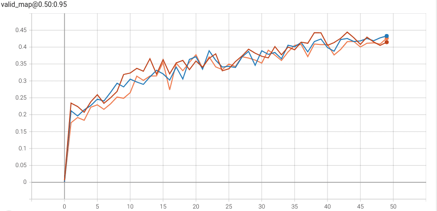
In the above graph:
- Red line: YOLO NAS Large model training
- Blue line: YOLO NAS Medium model training
- Orange line: YOLO NAS Small model training
The YOLO NAS large model reached the highest mAP of 44.4% on epoch 43. One more point to notice here is that the YOLO NAS Large model reached a higher mAP comparatively sooner. This indicates its capability to detect difficult objects in comparison to the YOLO NAS Medium and Small models.
The super-gradients API saves three different checkpoints for each experiment. One for the best model, one for the latest model, and one for the averaged weights.
As the YOLO NAS Large model performed the best during the custom dataset training, we will use that further for inference experiments.
Training YOLO NAS Large Model for Longer
From the above experiments, it is clear that the YOLO NAS Large model performs the best. To get even better results, we can train this model for 100 epochs. The YOLO_NAS_Large_Fine_Tuning.ipynb accomplishes this.
Here is the mAP graph after training the model for 100 epochs on the custom dataset.
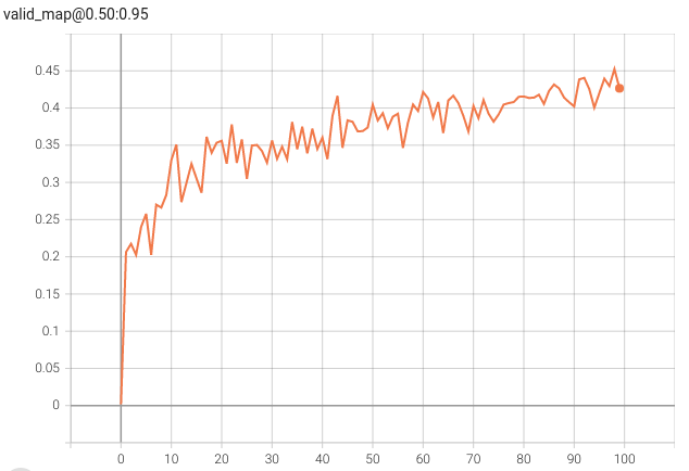
Fine-tuning the YOLO NAS Large model on the custom dataset achieves more than 45% mAP.
Inference on Test Images using the Trained YOLO NAS Model
The dataset contained a test split which we kept reserved for inference purposes. You can execute the code cells in the inference.ipynb notebook to run the inference experiment. It accomplices a few things:
- First, it loads the best trained YOLO NAS weights from the checkpoint directory.
- Then it runs the inference on the test images. While doing so, the code saves the inference results in the
inference_results/imagesdirectory with the original image names. - After obtaining the results, the notebook shows a set of images by overlapping the ground truth annotations on the predicted images.
The final step will tell us which objects the trained model missed and whether the model made any false predictions.
Let’s start our analysis by visualizing a few of the inference predictions.
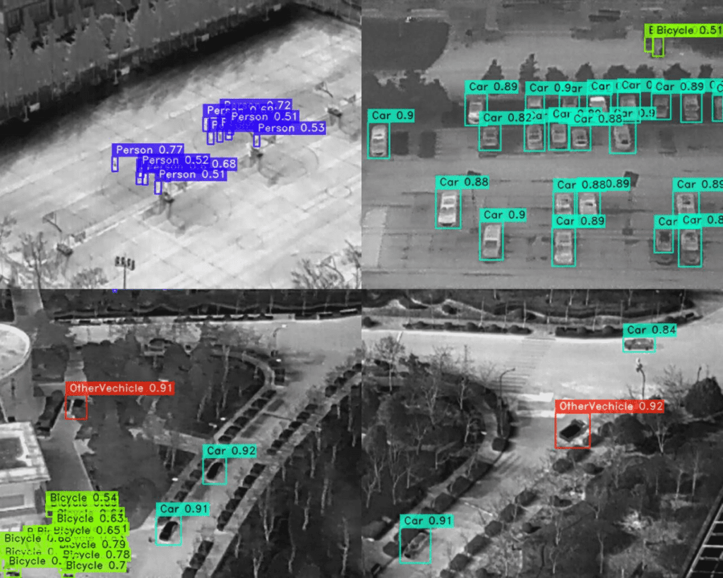
From a very initial analysis, it seems that the model predicts almost all the objects, even the persons, which appear very small. But it is extremely difficult to point out any mistakes here.
Visualizing the ground truth annotations on top of the predictions is a much better idea.
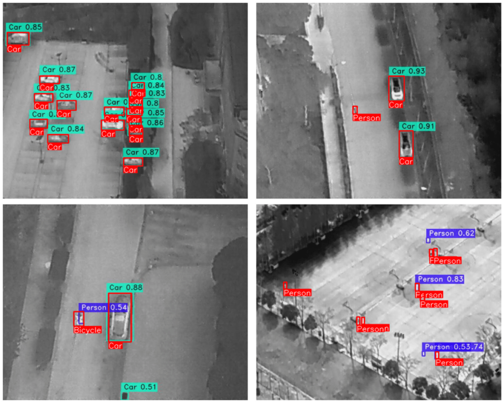
In the above images, the ground truth annotations are shown in red with the class names at the bottom.
We can see that in most cases, the model is missing detections for the Person class. Other than that, it detects an instance of a car that is not actually a car and also detects a Bicycle as a Person in one of the images.
Overall, the model is performing well and only fails to detect very difficult to recognize objects.
YOLO NAS Trained Model Video Inference Results
We also carried out an inference experiment on a drone thermal imaging video.
The results are quite impressive. The model can detect persons and cars in almost all the frames despite the shaky movement of the camera.
The video inference was run on a laptop with a GTX 1060 GPU, and the model ran at an average of 17 FPS. Given that we are using the YOLO NAS Large model here, we are getting decent speed.
Conclusion
In this article, we explore how to train the YOLO NAS models on a custom dataset. For our experiment, we chose a considerably challenging thermal imaging dataset with 5 classes. The objects in this dataset were small and difficult to detect for humans, but YOLO NAS did a very good job after fine-tuning it. This shows the potential of the YOLO NAS models for real-world use cases in detecting small objects in real time where the other object detection models may fail.
From the experiments, we can infer that the new YOLO NAS models open up a new world for real-time detection. These include surveillance, traffic monitoring, and medical imaging, among many others.
If you build your own applications using YOLO NAS or take this project further, let us know in the comment section. We will be happy to spread the word.
In case you missed it, here’s the complete list of posts from our YOLO series:
- YOLOv8 Ultralytics: State-of-the-Art YOLO Models
- Train YOLOv8 on Custom Dataset – A Complete Tutorial
- Deploying a Deep Learning Model using Hugging Face Spaces and Gradio
- YOLOv6 Custom Training for Underwater Trash Detection
- YOLOv6 Object Detector Paper Explanation and Inference
- YOLOX Object Detector and Custom Training on Drone Dataset
- YOLOv7 Object Detector Training on Custom Dataset
- YOLOv7 Object Detector Paper Explanation and Inference
- YOLOv5 Custom Object Detector Training on Vehicles Dataset
- YOLOv5 Object Detection using OpenCV DNN
- YOLOv4 – Training a Custom Pothole Detector
- YOLOR Paper Explanation and Comparison


