What is YOLO? You Only Look Once (YOLO): Unified, Real-Time Object Detection is a single-stage object detection model published at CVPR 2016, by Joseph Redmon, famous for having low latency and high accuracy. The entire YOLO series of models is a collection of pioneering concepts that have shaped today’s object detection methods.
YOLO Models have emerged as an industry de facto, achieving high detection precision with minimal computational demands. Some YOLO models are tailored to align with the specific processing capabilities of the device, whether it’s a CPU or a GPU. Most YOLO models are designed to cater to different scales, such as small, medium, and large, which can be easily serialized in ONNX, TensorRT, OpenVINO, etc. This gives users the liberty to choose which is best suited for their application.

There are limited resources on the internet that go through all the YOLO models, from their inner workings to how to train every model on the data of your choice end-to-end. However, in this article, we will go through all the different versions of YOLO, from the original YOLO to YOLOv8 and YOLO-NAS, and understand their internal workings, architecture, design choices, improvements, and custom training.
- Introduction to Object Detection
- Object Detection using Classical Computer Vision and Deep Learning
- One-Stage Vs. Two-Stage Detectors
- Challenges of Object Detection
- Introduction to YOLO
- Chronology of YOLO Models: Evolution and Milestones
- YOLO Controversy: Ethical Considerations and the Naming Saga
- YOLOv1
- YOLOv2
- YOLOv3
- YOLOv4
- YOLOv5
- YOLO-R
- YOLOX
- YOLOv7
- YOLOv6
- YOLOv8
- YOLO-NAS
- YOLOv9
- YOLOv10
- YOLO11
- YOLOv12
- Summary and Conclusion
- References
Introduction to Object Detection
Object detection is an important task in computer vision. In layman’s terms, Object detection is defined as Object Localization + Object Classification. Object Localization is the method of locating an object in the image using a bounding box and Object Classification is the method that tells what is in that bounding box.
There are numerous real-life applications for object detection. For example, in the field of Autonomous Vehicles, it is used for detecting vehicles, pedestrians, road delimiter prediction, HD-Map creation, traffic lights, and traffic signs, etc. In surveillance and monitoring, it is used in detecting trespassers, vehicle license plates, face mask detection, weapon detection etc. in biometric attendance systems. In medical imaging, its used for detecting certain cells, cancer detection, tumor detection, etc. and the list goes on.
Object Detection using Classical Computer Vision and Deep Learning
Earlier, detection algorithms used to be based on classical computer vision techniques such as template matching, Haar cascade, Feature detection and matching using SIFT or SURF, HOG Detector, Deformable Part-based Model (DPM), etc. However, most of these methods are very specific to the use case and don’t have generalization capabilities, which redirected the research toward deep learning-based methods. The Overfeat paper was a pioneer in deep learning-based object detection as it was a single network model employed to perform object classification and localization.
The Overfeat architecture closely resembles the AlexNet architecture. It does image classification on different scales in a sliding window fashion and carries out bounding box regression on the same CNN layer. Later other models like RCNN, FastRCNN, SPPNet, YOLO etc. emerged in this field.
One-Stage Vs. Two-Stage Detectors
Initial models were two-stage detectors, which means there was a step for region proposals and finding out the region of interest. It was also a step for predicting the bounding box coordinates and class using the proposed region. This was very innovative, yet it demanded substantial computational resources and resulted in considerable delays during the inference phase. Later the YOLO authors proposed a single-stage strategy that overlooked the Region Proposal step and ran detection directly over the entire image. This helped speed up the training and inference, preserve global context and keep the accuracy on par.
Challenges of Object Detection
1. Occlusion and Small Objects
Small objects are always difficult to detect because models get little information about them, or the dataset might not have many instances. This issue comes under the scope of shape invariance problem. Additionally, occlusion and partially visible objects make it hard for the model to detect small objects.
2. Global Context and Local Contexts
Global context is as important as local context for a model. Global context means the usual surroundings of the object, e.g. traffic light is mostly seen on the side of the road, or it might have cars or pedestrians nearby. The meaning of Local context is the object’s geometrical structure, texture, and colors. For instance, traffic lights typically appear rectangular, containing lights of various colors, red, green, or yellow. For the shape invariance property, a well-trained model doesn’t confuse a red light in a car’s rear as a red light from a traffic light. However, if the data is not properly curated, this issue might occur.
Introduction to YOLO
Chronology of YOLO Models: Evolution and Milestones
At CVPR 2016, Joseph Redmon, along with researchers from FAIR (Facebook AI Research) and the Allen Institute for AI, published the seminal paper on YOLO (You Only Look Once). It was a state-of-the-art, single-stage object detector at that time. Using the same concept of single-stage detection along with some significant changes, people published their own models, such as SSD, RetinaNet, etc.
At the 2017 CVPR, Joseph Redmon and Ali Farhadi published the 2nd iteration of the YOLO model as YOLOv2, built on top of YOLOv1, integrating some advancements of that time to make it faster and more accurate. Redmon improved the architecture by adding a Neck and using a bigger backbone and published a very casually written paper in ArXiv in 2018.
Two years later, in April 2020, other authors used the YOLO name to publish version 4 of the model and a lot of significant changes were made. Two months later, Ultralytics open-sourced the YOLOv5 model but didn’t publish any paper. In the same year, YOLOv4 authors published another paper named Scaled-YOLOv4 which contained further improvements on YOLOv4. In the following year, 2021, YOLOR and YOLOX were published. Skipping version 6, in 2022, the authors of YOLOv4 published the YOLOv7, which was the state of the art at that time in terms of speed and accuracy. In the same year, researchers from Meituan Vision published the YOLOv6, which was better than version 7.
In January 2023, Ultralytics open-sourced the YOLOv8 with instance segmentation capabilities alongside detection. In May 2023, Deci AI came up with YOLO-NAS, an algorithm-generated architecture that surpassed all the predecessors of YOLO.
YOLO Controversy: Ethical Considerations and the Naming Saga
In February 2020, Redmon tweeted that he stopped researching computer vision because of the concerns that his research was bringing in military applications and privacy concerns. Growing up, he believed that science was independent of political views and the act of conducting research was inherently ethical and beneficial, regardless of the topic. His purpose was to share his point of view about one of the NeurIPS guidelines emphasizing the social benefit of research.
I stopped doing CV research because I saw the impact my work was having. I loved the work but the military applications and privacy concerns eventually became impossible to ignore.https://t.co/DMa6evaQZr
— Joseph Redmon (@pjreddie) February 20, 2020
After that, everyone questioned whether YOLO was a good name for a series. Some also called the YOLOv4 “The last YOLO.”
Almost two years had passed since YOLO released its last model. It was not until April 2020 that Bochkovskiy et al. published their work as YOLOV4. He was also a DarkNet maintainer. In light of the tweet from Redmon, it appeared that the authors of YOLOv4 did not consult with Redmon or other authors before publishing their work under the name YOLO.
Nevertheless, Redmon understood the hard work put into YOLOv4 and did not shy away from acknowledging it. Looking at the satisfactory improvements, the CV community also accepted the work as the official YOLOV4.
Doesn’t matter what I think! At this point @alexeyab84 has the canonical version of darknet and yolo, he’s put a ton of work into it and everyone uses it, not mine haha. https://t.co/FcnQPiySr7
— Joseph Redmon (@pjreddie) April 25, 2020
In May 2020, Glenn Jocher created a repository named YOLOV5 under the Ultralytics Organization on GitHub. In June 2020, he pushed his first commit on that repository with the message “YOLOv5 Greetings”. The code was ported to Pytorch from the Darknet framework.
YOLOv5 contained a lot of improvements from the YOLOV4 model, no paper was published, and it marked the first instance of a YOLO model that did not use the DarkNet framework for its development, which started a debate about whether Glenn was justified in releasing the model under the YOLO name. At that time, Roboflow also published an article comparing YOLOV5 and YOLOV4, which trended on HackerNews and fueled the debate. Everyone started talking about this on Reddit, Twitter, and even GitHub. On June 14th, 2020, in a GitHub issue thread, Glenn Jocher stated that he would publish a summary of YOLOv5, by the end of 2020, On November 2023, they published a short synopsis.
Later, many folks started borrowing the name YOLO for their model(which was, in a way, an improvement to the original model). On the one hand, allowing researchers to use the name helped in the development of YOLO model around the globe. Still, it made it difficult to keep track of the progress because people continued improving on their old contributions. For example, you can’t understand YOLOv7 if you read YOLOv5 or YOLOv6, to understand that, you need to follow the authors and see what they published before the current paper, which was YOLOv4-Scaled, YOLO-v4, and CSPNet.
YOLOv1
Paper Summary
- Generally, there are two types of Deep Learning object detection models: single-stage and two-stage models. The single-stage model follows a specific design pattern, which is the Backbone-Neck-Head. However, in YOLOv1, there is no concept of a neck, only a backbone and head. YOLOv1 architecture is inspired by GoogleNet’s architecture, and has 24 convolutional layers and two fully-connected layers. In these layers, the first twenty layers act as a backbone, and rest of the layers lead up to an additional two fully-connected layers, acting as a detection head. Instead of the inception module, they used a 1×1 convolution layer with 3×3 convolutional layers in the backbone. This helped to reduce the number of channels without having to reduce spatial dimensions, and the number of parameters became relatively low.

- The authors of YOLOV1 pre-trained the first 20 layers of YOLO in ImageNet at a resolution of 224×224, and the four remaining layers were finetuned in PASCAL VOC 2012 at a resolution of 448×448. This increased the information for the model to detect small objects more accurately. They trained their model for 135 epochs on the training and validation sets from VOC 2007 and 2012. They used a batch size of 64, momentum of 0.9, and learning rate decay of 0.0005. The learning rate(LR) scheduling is such that in the first few epochs the LR rate rises from
 to
to  . Initially it is trained for 75 epochs with a learning rate of
  followed by
  for 30 epochs, and finally the model undergoes an additional
  for 30 epochs.
- To avoid overfitting, the authors used a dropout rate of 0.5 and extensive augmentation. Scaling and translations of up to 20% of the total dataset were used. They randomly adjusted the exposure and saturation of the image by up to a factor of 1.5 in the HSV color space. A linear activation function was set for the final layer, and the rest of the other layers used the leaky-ReLU activation.
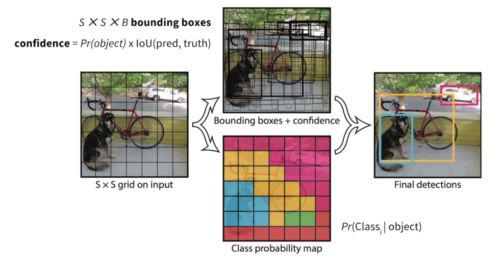
- There is no concept of anchor-free boxes. The authors divided the image into an SxS grid, where each grid predicts B bounding box coordinates and an objectness score associated with bounding boxes and C number of class probabilities. The prediction gets encoded in a
 tensor. It also means that One grid cell can only predict one object. As bounding box coordinates, YOLO predicts the center (x,y) of the bounding box and the width(w) and height(h) of the box. The center is relative to the grid cell, so it’s between 0 and 1, and width and height are relative to the image size, which also comes in the range of 0 and 1. Objectness score refers to the score that tells if a bounding box contains an object or not, which is denoted as
  , where
  is the probability to have an object in the cell and
  is the intersection over union between predicted region and the grand truth.
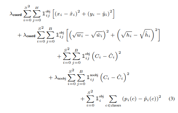
- As the detection head needs to predict the bounding box coordinates, objectness score, and object class, they have three parts to the loss function: localization loss, confidence loss, and classification loss. As the object detection was depicted as a regression problem, all losses are sum-squared errors. The first two loss terms belong to localization loss, the next two losses belong to the confidence loss, and the last one belongs to the classification loss. Often there are grids that don’t predict any bounding box, which pushes the confidence score of those cells toward zero, overpowering the cells that contain an object. Two parameters
 and
and  were proposed to resolve this issue.
YOLOv2
Paper Summary
YOLOv2 was published at CVPR, in 2017, by the same YOLOv1 authors. They slightly modified the YOLOv1 architecture and improved the training process to make YOLOv2 faster and more accurate. Here are the changes that enhanced YOLOv2.
Using High-Resolution Images:
They trained their classification network at 448×448 in ImageNet for 10 epochs. This helps the network to adjust the filters to better work with high-resolution images. Later, the resulting network is trained on detection tasks, and by doing that, they promote joint training that helps train object detectors in both object detection and classification data. Their objective mainly was improving recall and localization while maintaining classification accuracy. They use 416×416 instead of 448×448 so that feature maps are sized in odd numbers, and the object center should lie at one point instead of multiple locations. YOLO’s convolution layers downsample the image by a factor of 32, so by using an input image of 416, we get an output feature map of 13 × 13.
Introduction to Anchor Boxes:
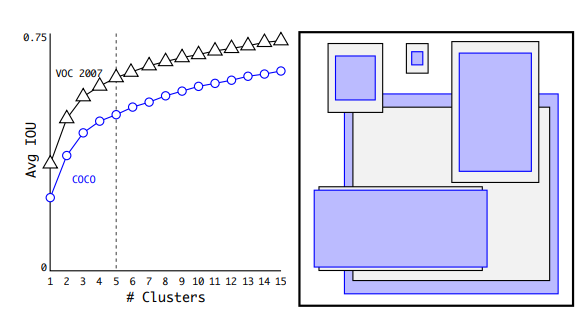
Generally, the box dimensions are hand-picked, which is only sometimes a good prior. To solve this, the authors proposed using k-means clustering on all the bounding boxes of the dataset. This gives them the most dominant sizes of the bounding boxes from the dataset. But, in k-means, using Euclidean distance will produce a higher error(distance) for large boxes and a more minor error(distance) for small boxes. But, as the IOU score is independent of the size of the box, the distance measurements needed to be changed. They proposed,

This part of the equation implies that the distance is inversely proportional to the IOU. Subtracting the IOU from 1 means that the distance decreases as the IOU increases (indicates higher overlap or similarity), and vice versa. They ran k-means for various values of k and plot the average IOU with the closest centroid, see Figure 6. and chose k = 5 as a good tradeoff between model complexity and high recall.
Fine-grained features:
Like YOLOV1, YOLOV2 also predicts the bounding box coordinates relative to the grid cell. The modified YOLO predicts a 13×13 feature map, and while this helps detect large objects, having a fine-grained feature map might help detect small objects. Many detection models have different approaches, but in YOLOv2, the authors proposed a passthrough layer that concatenates features from a higher resolution layer to a lower resolution layer. When concatenating a higher-resolution image with a lower-resolution image, it internally restructures the higher-resolution image such that the spatial dimension reduces, but the depth increases. This means that if given a 26x26x512 feature map, it gets resized as 13x13x2048; here, the channel dimension 2048 comes from 512 x 2 x 2 = 2048.
Location Prediction:
The diagram below is explained as,
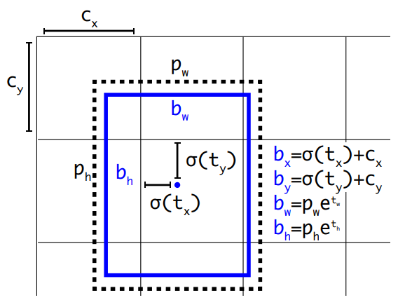
Here, ![]() ,
, ![]() is the grid cell center.
is the grid cell center. ![]() ,
, ![]() are the coordinates of the center of the predicted bound box relative to the grid cell.
are the coordinates of the center of the predicted bound box relative to the grid cell. ![]() and
and ![]() are the width and height of the predicted bounding box, which is an offset of the prior anchor box associated with the grid. σ ensures the center point (
are the width and height of the predicted bounding box, which is an offset of the prior anchor box associated with the grid. σ ensures the center point (![]() ,
, ![]() ) stays within the grid cell by restricting the values between 0 and 1.
) stays within the grid cell by restricting the values between 0 and 1. ![]() and
and ![]() represent the exponential transformation of predicted width and height offsets
represent the exponential transformation of predicted width and height offsets ![]() and
and ![]() , ensuring that the width and height stay positive, although using an exponential transform is mathematically unstable.
, ensuring that the width and height stay positive, although using an exponential transform is mathematically unstable.
Multiscale training:
They introduced multiscale training to make the model more robust. After every 10 batches, the model takes a randomly selected image dimension and continues training. Since their model downsamples by a factor of 32, they pull from the following multiples of 32: {320; 352; …; 608}.
Hierarchical classification:
The model is first trained for classification on ImageNet before even training detection. For that, they hierarchically prepare their data. Hierarchical Classification improves the model accuracy by leveraging the structure of class label’s hierarchically, the model can better understand the relationships between different classes.
YOLOv3
Paper Summary
- In YOLOv2, the model predicts the object class for each grid. But, in YOLOv3, the model predicts class for each bounding box predicted. The model predicts 3 bounding boxes for each grid, objectness score, and class predictions. At the output side, the tensor is of
 . The model outputs bounding boxes at three different scales.
 - YOLOv3 uses multiple independent logistic classifiers rather than one softmax layer for each class. During training, they use binary cross-entropy loss in a one vs. all setup.
- YOLOv3 uses the DarkNet-53 as a backbone for feature extraction. The architecture has alternative 1×1 and 3×3 convolution layers and skip/residual connections inspired by the ResNet model. They also added the idea of FPN to leverage the benefit from all the prior computations and fine-grained features early on in the network. Although DarkNet53 is smaller than ResNet101 or RestNet-152, it is faster and has equivalent or better performance.
- Similar to YOLOv2, YOLOv3 also uses k-means to find the bound box before the anchors. In this model, they used three prior boxes for different scales, unlike YOLOv2.
Training YOLOv3
Ultralytics has a YOLOv3 repository that is implemented in Pytorch. They provide a command line interface to train a model swiftly. The official repository for YOLOv3 is in the darknet framework. YOLOv3 custom training is a good resource to understand how scratch training works. We also show the training of YOLOv3 using Opencv python and c++ on the coco dataset.
YOLOv4
Paper Summary
- Alexey Bochkovskiy collaborated with the authors of CSPNet(Nov 2019) Chien-Yao Wang and Hong-Yuan Mark Liao, to develop YOLOv4. The only similarity between YOLOv4 and its predecessors was that it was built using the Darknet framework. They experimented with many new ideas and later published them in a separate paper, Scaled-YOLOv4.

- Generally, an object detector comprises an ImageNet pre-trained backbone for feature extraction and a Head for doing the bounding box regression and classification. But, from YOLOv3 and YOLOv4, the authors introduced another part of the structure called the Neck, placed between the backbone and the head. The use of this block is to collect features of different stages from the backbone and pass them to the head. In YOLOv4, we had CSPDarkNet53 as the backbone, Spatial Pyramid Pooling (SPP), and Modified PANet as the Neck and the YOLOV3 head. In the paper, they introduced two concepts: bag of freebies and bag of specials. The concept of “Bag of Freebies” refers to techniques that modify the training approach or raise the training cost without affecting the cost during inference. Data augmentation is a typical example of such a method. In contrast, “Bag of Specials” includes methods that marginally increase the cost at inference time but substantially enhance accuracy. These methods involve expanding the receptive field, integrating features, and various post-processing techniques. Specific examples like SPP (Spatial Pyramid Pooling) and PANet (Path Aggregation Network) were elaborated on in the YOLOv5 section.
- Cross Stage Partial Network was designed for faster inference while keeping the accuracy of the original model. It is an additional component that can be integrated into your existing setup. The concept behind CSPNet is that architectures like ResNet and DensNet have many skip connections. A large amount of gradient information is reused during the gradient updation of different layers, which results in different layers repeatedly learning copied gradient information. To stop this duplicate gradient, CSPNet divides the input into two parts, one passes through the usual in-between layer, and the 2nd part gets concatenated after that block for further operations.
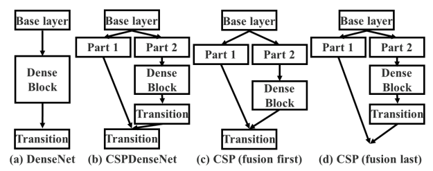
- The authors experimented with many architectures such as ResNet50, ResNext50, VGG16, DarkNet53, etc., but later, a variant of DarkNet53 with the CSPNet was used for the backbone. Numerous studies demonstrated that the CSPResNext50 was better than CSPDarkNet53 for object classification. However, through experimentation, they discovered that the CSPDarkNet53 is more suited for Object Detection tasks.
- They introduced Spatial Pyramid Pooling(SPP) as in YOLOV3-SPP for the multi-scale feature pooling. They use PANet for the feature pyramid instead of FPN from the YOLOV3 model. In the literature, two types of attention modules used in an object detector are channel-wise attention and point-wise attention. Spatial Attention Module (SAM) and Squeeze-and-Extraction are examples, respectively. SAM is used in YOLOv4 because it improves accuracy and decreases the inference latency. Finally, for the detection head, they use anchors as in YOLOv3. Above mentioned integrations are a part of the bag of specials, where CSPNet cuts the computations cost while maintaining the accuracy, SPP block helps to increase the receptive field, and PANet helps for better feature aggregation.
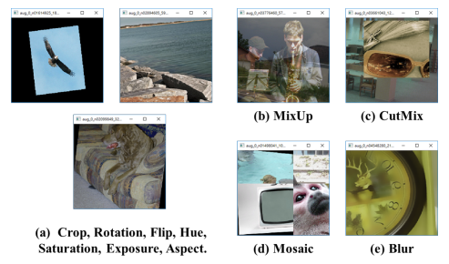
- As a bag of freebies method, the authors introduced the mosaic data augmentation, which combines 4 images in one image. By doing that, they add contextual information and decrease the mini-batch size for batch normalization. They also used MixUp and CutMix alongside other geometrical augmentations except for mosaic. They used cIOU loss and cross mini-batch normalization for better detection, replacing normal Dropout with the DropBlock.
Training YOLOv4
Custom training of YOLOv4 on pothole detection involves using YOLOv4 and the darknet framework. The dataset contained 1265 training images, 401 validation images, and 118 validation images.
YOLOv5
Paper Summary
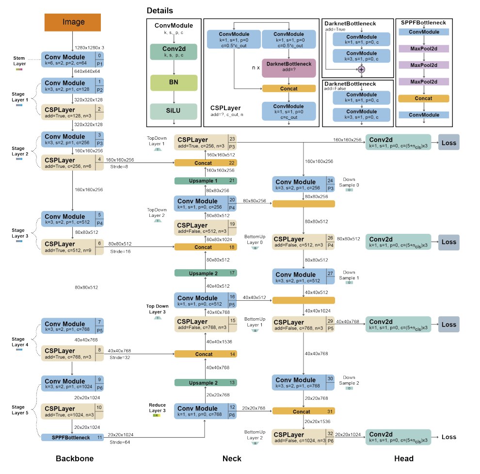
Model Architecture:
The YOLOv5 model is divided into 3 parts, Backbone, Neck, and Head. Each convolution is followed by batch normalization (BN) and SiLU activation. Below is the 1000-feet overview of the YOLOv5 Model Architecture
- Backbone: CSP-DarkNet53
- Neck: SPPF and CSP-PANet
- Head: YOLOv3 Head
Spatial Pyramid Pooling Fast (SPPF):
SPPF is one of the improvements that they introduced in their model. This is nothing but SPP, it’s just that instead of passing the input to three different max-pool layers, the output of one max-pool block is being fed to the subsequent max-pool layer, which makes the process much faster. Below is the Pytorch implementation of SPP and SPPF:

PANet (Path Aggregation Network):
PANet was used in YOLOv4. The aim of using PANet was to create a rich multi-stage feature hierarchy for robust object detection. The only modification is that PANet concatenates the feature maps instead of adding them, as mentioned in the original paper. CSP-PANet is the same as PANet. Instead, they add a few CSP layers in between the PANet. This change results in a processing speed that is more than twice as fast.
AutoAnchors:
YOLOv5 also incorporated another improvement which is called AutoAnchor. In AutoAnchor, they change the shape of the anchors during training. First, the model starts with the prior anchor boxes generated from running k-means on the ground truth bounding boxes. Later these bounding boxes get updated using the genetic evolution (GE) algorithm. GE algorithm develops these anchors across 1,000 generations, employing CIoU loss and the Best Possible Recall for its fitness evaluation.
Bag of freebies:
Apart from this bag of special methods, they also used the bag of freebies methods and data augmentations such as Mosaic, copy-paste, random affine, MixUp, HSV augmentation, etc. I remember from the TensorFlow – Help Protect the Great Barrier Reef Kaggle competition, where people suddenly started training YOLOv5 on high-resolution images, which resulted in higher Leader Board scores. However, it was later tested that using a larger input size of 1536 pixels and test-time augmentation (TTA), YOLOv5 achieves an AP of 55.8%.
Training YOLOv5
YOLOv5 stands out as a top-performing version in the YOLO series, and mastering its training on custom datasets is essential. Training YOLOv5 on the vehicle OpenImage dataset serves as a practical example. The transition of the model from the darknet framework to Pytorch by Glenn Jocher has simplified the training process significantly. For those looking to delve deeper, “YOLOv5 – Custom Object Detection Training” offers comprehensive insights into custom training techniques. Understanding the deployment of models in edge devices, particularly running YOLOv5 with OpenCV in Python and C++, is crucial for practical applications. Additionally, Ultralytics has recently introduced the capability to train instance segmentation models using the YOLOv5 repository, a feature explored in detail in “YOLOv5 Instance Segmentation“.
YOLO-R
Paper Summary
- In mid-2021 a few authors from the YOLOv4 team published YOLO-R. With this paper, the authors started exploring along the lines of multi-task learning.
- The authors found that the feature extracted for a specific task is not generalized enough to be applied to other tasks. This means one can’t directly use the features from a detection model in a segmentation model. To solve this, everything boils down to producing a generalized representation. And this is where Multi-task Learning(MTL) comes into the picture. In MLT the model is trained to perform multiple different tasks simultaneously, rather than training task-specific models. By parallel training a model for multiple tasks, one can improve the model’s generalization capabilities. This is because the model leverages the commonalities and differences across the tasks. MLT is also helpful because it reduces the number of model parameters, resulting in fewer FLOPs and a decreased model latency.
- The concept of YOLOR is not like usual MLT models, where you see shared representation components, task-specific components, rather, the concept of YOLOR comes from implicit knowledge and explicit knowledge. Knowledge is two types: explicit knowledge and implicit knowledge. Humans learn by looking, hearing, tactile, etc., which are a type of explicit knowledge, and they also learn from past experiences, which is categorized as implicit knowledge. Implicit knowledge refers to the knowledge learned in a subconscious state.
- In terms of neural networks, there will be a network for learning explicit knowledge, and there will be another model jointly trained with the explicit model for learning implicit knowledge. In this diagram, the authors presented the same concept,
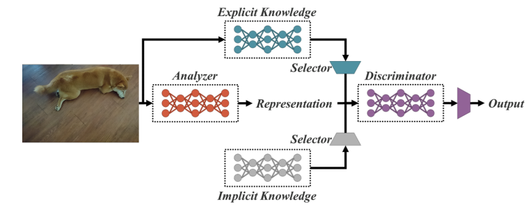
- For the Explicit knowledge network, the authors used YOLOv4-Scaled with a slight modification of adding a reOrg Layer followed by two convolution layers. In the Implicit network, they used a single convolutional layer with two learnable priors for kernel space alignment and prediction refinement. They included object detection, multi-label image classification, and feature embedding for multi-task learning.
- For further understanding YOLOR comprehensive paper review is a very good resource that goes over Implicit and explicit knowledge in depth, how humans understand and learn, how to model implicit knowledge, how to combine that with explicit knowledge to improve model capabilities, and so on.
YOLOX
Paper Summary
- In July 2021, YOLOX was published by Megvii Technology, China. This model was the first-place winner of the Streaming Perception Challenge of the WAD workshop at CVPR 2021. It was published on the same timeline as YOLO-R. When the authors of YOLOR tried to explore multi-task learning, the authors of YOLOX focused on integrating the recent advances into the YOLO model. All YOLO models before YOLOX were using Anchor boxes. However, during that period, most state-of-the-art models used Anchor-free detectors. Hence, the authors incorporated this approach into their model, along with the advanced label assignment strategy simOTA, Decoupled Head, and Strong Augmentations.
- The YOLOX model features the DarkNet53 from YOLOv3 with spatial pyramid pooling(SPP) as the backbone, FPN as the Neck, and a customized decoupled head. The YOLOX model was trained from scratch, the authors excluded ImageNet Pre-training because using that with strong augmentations was no longer useful. At that time, YOLOv3 was still one of the best detectors to which a large part of the industry could turn because of limited computation. YOLOv5, on the other hand, was optimized, keeping the anchor-based method in mind. Although the Backbone and Neck of the YOLO detectors improved over time, the head part was untouched, and decoupling the head also resolved the long ongoing conflict of classification, and regression tasks. This helped them in faster convergence.
- It starts with one 1×1 conv layer, two 3×3 conv layers again, and a 1×1 conv layer (for each branch). They had a very good training regimen, 300 epochs of training with SGD, cosine scheduler, multi-scale training, EMA weight updation, BCE loss for the classification branch, and IoU loss for the regression branch.
- The authors used heavy augmentations to improve the model performance, they explicitly added the famous Mosaic and MixUp in their augmentation pipeline. They found out that for large models, strong augmentation was useful. They used MixUp with scale jittering in their pipeline after exterminating with MixUp and Copypaster.
- Inspired by end-to-end (NMS-free) detectors, the authors added two additional convolution layers, one-to-one label assignment and stop gradient. Still, unfortunately, that slightly decreased the performance and the inference speed, so they dropped it.
Training YOLOX
YOLOX, a model meticulously engineered for object detection, has been effectively utilized for YOLOX custom training on the Drone Detection dataset, featuring 4014 labeled images. The training was conducted using the official YOLOX repository, with the model being tested in various configurations to analyze its performance. The outcomes of these tests are shared to provide insights into the model’s capabilities.
YOLOv7
Paper Summary
The YOLOv7 is the continuation after Scaled-YOLOv4. YOLOv4 and YOLOv7 are published by the same authors. The YOLOv7 model introduces novel modifications such as E-ELAN, Model Scaling, Planned re-parameterized convolution, Coarse for auxiliary, and penalty for lead loss.
Extended-ELAN (E-ELAN):
E-ELAN is an Extended efficient layer aggregation network, a variant of ELAN. ELAN is inspired by VoVNet and CSPNet. We already know about CSPNet, and VoVNet is nothing but an Object Detection Network composed of cascaded OSA modules. OSA means One-shot Aggregation. It is more efficient than Denses Block in DenseNet and optimized for GPU computation. The below image clears the concept of OSA,

It is similar to DensesNet, but we concatenate the features after a few conv blocks here.
Compound Model Scaling:
The authors used model scaling to adjust parameters to generate models of different scales. By different scales, it means a change in model parameters. It helps to meet the need for different inference speeds. In EfficientDet, scaling is done in width, depth, and resolution, and Scaled-YOLOv4 scales the model in stages (No. of feature pyramid). In this model, they used NAS (Network Architecture Search), which is a commonly used model scaling method, authors also showed that this method can be further improved using the compound model scaling approach.
Model Re-parameterization:
Model re-parameterization means model weight averaging. There are two ways of doing model averaging,
- Averaging the weights of the same model trained on different folds of data.
- Averaging the model weights of different epochs.
This is a very popular ensemble technique. Pytorch has an implementation of the same named SWA(Stochastic Weight Averaging).
Coarse for Auxiliary and Fine for Lead Loss:
As you can see, the model architecture has multiple heads predicting the same thing. The head responsible for the final output is the lead head, and the other heads assist in the model training. With the help of an assistant loss, the weights of the auxiliary heads are updated.
For a deeper comprehension of the YOLOv7 paper and its inference outcomes, YOLOv7 Paper Explanation is an invaluable resource. It offers a thorough analysis and provides critical insights, enhancing understanding of the subject matter.
Training YOLOv7
The process of YOLOv7 fine-tuning was demonstrated using the pothole dataset with the official YOLOv7 repository. This included both fixed-resolution and multi-resolution training, accompanied by an in-depth analysis of model inference. Additionally, a detailed comparison of GPU and CPU performances was conducted in the study of YOLOv7 and media pipe human pose estimation, offering valuable insights into their respective efficiencies.
YOLOv6
Paper Summary
- Two months after the YOLOv7 release, researchers from Meituan Inc, China, released YOLOv6. Yes, you heard it right, YOLOv7 was published before YOLOv6. And apparently the authors took permission from the original YOLO authors. YOLOv6 was the state-of-the-art(SOTA) when it was published.
- In this paper, the authors experimented with many techniques, and the resulting successful methods were integrated with the model and published as YOLOv6. YOLOv6 is an anchor-free, decoupled head architecture with a unique backbone named EfficientRep.

- EfficientRep consists of a RepVGGBlock stem, followed by 4 blocks of ERBlock. ERBlock is made of a RepVGGBlock and a RepBlock. The last layer of ERBlock has a RepVGGBlock and RepBlock, with the exception of SimSPPF, which is nothing by the SPPF layer with ReLU activation. For Neck, they used Rep-PAN, which is nothing but the good old PANet from YOLOv4 and YOLOv5, it is just that we replace the CSPBlock with RepBlock (for small models) or CSPStackRep Block (for large models). For Head, they used a customized version of the decoupled head from YOLOX, which they named the hybrid-channel strategy. In this method, they reduced one 3×3 conv layer and jointly scaled the width of the head by the width multiplier for the backbone and the neck.
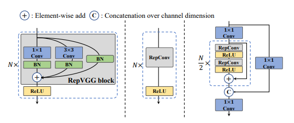
- Except for these architectural changes, they used advanced Label Assignment techniques such as simOTA, and TAL(Task alignment learning), a lot of new loss functions were introduced, and to make the model faster and more accurate, they used a lot of post-training quantization methods, such as self-distillation, Reparameterizing Optimizer, etc.
- YOLOv6 is a very important addition to the YOLO series of models, and it’s very important to understand what improvements were made to make the model more efficient. YOLOv6 – Paper Explanation is a great resource to understand YOLOv6 thoroughly; it meticulously clarifies complex concepts such as RepConv, RepVGGBlock, CSPStackRep, VFL, DFL, and Self-Distillation very carefully.
Training YOLOv6
- Although it’s named YOLOv6, it was the best-performing model when it was published. And it is very crucial to understand how to train a YOLOv6 on a custom dataset. YOLOv6 custom dataset training for Underwater Trash Detection provides an excellent guide for such custom training applications.
Comparison Between YOLOv5, YOLOv6, and YOLOv7
So far, we’ve thoroughly examined various models to understand their performance capabilities. However, there’s more to selecting the ideal model than just accuracy. Factors like inference speed on CPUs and GPUs, frames per second (FPS) rates, and choosing the right variant (Tiny, Small, Medium, or Large) are crucial for optimal model selection. A detailed comparison of YOLOv5, YOLOv6, and YOLOv7 provides an invaluable resource in this regard. This comprehensive analysis dives deep into each model’s specifics, covering all these important aspects to help you get answers and decide.
YOLOv8
Paper Summary
- In January 2023, Ultralytics came up with YOLOv8, which was the SOTA at that time. The model was open-sourced, but the maintainers didn’t publish any paper. Looking at the architecture of the YOLOv8 model, the previous model seemed over-engineered.

- The YOLOv8 architecture follows the same architecture as YOLOv5, with a few slight adjustments, such as the use of the c2f module instead of CSPNet module, which is just a variant of CSPNet, (CSPNet followed by two convolutional networks). They designed YOLOv8 anchor-free using YOLOv5 as a based model, which YOLOX authors tried but ended up using YOLOv3 as they found YOLOv5 over-optimized for anchor-based training. They also introduced Decoupled heads to independently process objectness, classification and bounding box prediction tasks. They used the sigmoid layer as the last layer for objectness score prediction and softmax for classification.
- YOLOv8 uses CIoU and DFL loss functions for bounding box loss and binary cross-entropy for classification loss. These losses have improved object detection performance, particularly when dealing with smaller objects. They also introduced the YOLOv8-Seg model for semantic segmentation by applying minimal changes to the original model.
- The absence of an official paper for YOLOv8 poses challenges in understanding the intricacies of the model through code or GitHub discussions alone. To bridge this gap, YOLOv8: A Comprehensive Guide emerges as a pivotal resource, offering in-depth insights and explanations about YOLOv8.
Training YOLOv8
The YOLOv8 model custom training was demonstrated using the Ultralytics repository, utilizing a diverse pothole dataset compiled from Roboflow, Research-Gate, manually annotated YouTube videos, and the RDD2022 dataset. This training involved a total of 6962 images for training and 271 for validation. Furthermore, for those interested in a different approach, there is a guide on training YOLOv8 using KerasCV. The article also delves into a comparative analysis of various YOLOv8 variants alongside their inference results. Additionally, YOLOv8’s capability for semantic segmentation, with minimal modifications to its original detection architecture, is detailed in YOLOv8 Instance Segmentation Training on Custom Data.” For exploring applications beyond object detection, YOLOv8 Animal Pose Estimation provides valuable insights into fine-tuning YOLOv8 for pose estimation tasks in the realm of computer vision.
Comparison of YOLOv8 Variants
We also have an in-depth article on comparing YOLOv8 models of different scales on the Global Wheat Data 2020 dataset. Here, we have discussed a comparative analysis of variously sized YOLOv8 models available in KerasCV.
YOLO-NAS
Paper Summary
In May 2023, an Israel-based company Deci, published their latest YOLO variant called YOLO-NAS, the current state-of-the-art object detection model. YOLO-NAS is tailored for efficiently detecting small objects and boasts enhanced localization precision. It also improves the performance-to-compute ratio, making it ideal for real-time edge-device applications.
They introduced a few quantization-aware modules, such as QSP and QCI. The architecture was generated through AutoNAC, which is Deci’s proprietary NAS technology. NAS means Neural Architecture Search. YOLO-NAS models incorporate attention mechanisms and reparameterization during inference to enhance their ability to detect objects.
- The YOLO-NAS models initially underwent pre-training on the Object365 benchmark dataset, which contains 2 million images across 365 categories.
- They were further pre-trained using a method called pseudo-labeling on 123,000 unlabeled images from the COCO dataset.
- Additionally, techniques like Knowledge Distillation (KD) and Distribution Focal Loss (DFL) were employed to refine and enhance the training process of the YOLO-NAS models.
- They generated different variants of YOLO-NAS by varying the depth and positions of the QSP and QCI blocks.
- YOLO-NAS and AutoNAC are very highly sophisticated algorithms, YOLO-NAS Object Detection Model serves as an informative resource to comprehensively understand the intricacies of this model.
Training YOLO-NAS
YOLO-NAS, one of the newest members of the YOLO family, is essential for those looking to Train YOLO-NAS on a custom dataset. We have illustrated this process using a Thermal Dataset. In addition to object detection, the YOLO-NAS series also excels in pose estimation, with YOLO-NAS Pose an excellent guide for a comprehensive understanding of its mechanics and applications.
YOLOv9
The paper introduces Programmable Gradient Information (PGI) and a new network architecture called Generalized Efficient Layer Aggregation Network (GELAN) to address data loss issues in deep learning networks during feature extraction and transformation. PGI is designed to preserve complete input information for reliable gradient calculations, enhancing weight updates. GELAN utilizes conventional convolution over depth-wise convolution for better parameter efficiency.
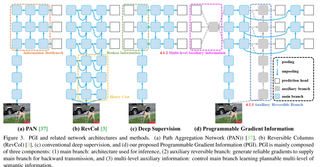
The issue of information loss, as described by the Information Bottleneck Principle, is significant in deep neural networks, leading to unreliable gradients and poor convergence. The paper suggests reversible functions to maintain information integrity throughout the network layers, improving training effectiveness.
PGI integrates a main inference branch, an auxiliary reversible branch, and multi-level auxiliary information. The reversible branch helps retain complete data information, reducing the risk of false correlations and enhancing parameter learning without increasing inference costs, as it can be omitted during inference. The multi-level auxiliary information integrates gradient information across various prediction branches, ensuring comprehensive learning across different targets.
Experimentally, YOLOv9, utilizing GELAN and PGI, outperforms other real-time object detectors in terms of accuracy and efficiency. It surpasses models that use depth-wise convolution or rely on ImageNet pretraining. The success of YOLOv9 is attributed to its superior parameter utilization and the ability of PGI to retain crucial information for effective data-target mapping.
Furthermore, CSP blocks within GELAN enhance performance with fewer parameters, allowing for a flexible yet stable architecture design. PGI’s integration with deep supervision concepts also shows marked improvements, particularly in deep models.
Training YOLOv9
Shortly after YOLOv9 was published, we released an introductory article that talks about the intricate workings of YOLOv9 in detail. Understanding how to adapt this model for use with your custom data is crucial. To assist with this, we crafted the article “Fine-Tuning YOLOv9 Models on Custom Dataset.” Following this, we also published an interesting article on training custom datasets for instance segmentation with YOLOv9, and we compared the outcomes with those from YOLOv8.
YOLOv10
Paper SummaryYOLOv8 architecture: yolo multiple object detection
While previous versions, including YOLOv9, introduced advancements like Programmable Gradient Information (PGI) and Generalized Efficient Layer Aggregation Network (GELAN) to improve computational efficiency, they still relied on Non-Maximum Suppression (NMS) for post-processing. This reliance hindered end-to-end deployment and increased inference latency.
YOLOv10 introduces two fundamental upgrades over its predecessors:
- Consistent Dual Assignments for NMS-Free Training
- Efficiency-Accuracy Driven Model Design

assignments in Top 1510
These innovations significantly enhance performance, computational efficiency, and accuracy, making YOLOv10 a breakthrough in real-time object detection.
NMS-Free Training and Inference
YOLOv10 eliminates the need to filter redundant bounding boxes by adopting an NMS-Free training paradigm inspired by DETR-style architectures. It consists of two main components: a Dual Label Assignment using two heads and a Consistent Matching Metric to match both head predictions for a perfect prediction.
Dual Label Assignments
YOLOv10 introduces a dual-head approach to optimize label assignments:
- One-to-Many Head: Provides dense supervision by retaining the original training objectives.
- One-to-One Head: Ensures a strict one-to-one mapping between predictions and ground truth, eliminating the need for NMS during inference. This is similar to Hungarian Matching but optimized for efficiency.
Consistent Matching Metric
A consistent matching metric aligns the training objectives of the one-to-many and one-to-one heads. This metric ensures that the best predictions chosen by one-to-many supervision are also valid for the one-to-one head, improving overall model performance. The alignment minimizes the supervision gap, leading to better predictions and lower inference latency.
Efficiency-Driven Model Design
YOLOv10 employs a holistic efficiency-accuracy-driven design to reduce computational costs while maintaining high accuracy. This is achieved through several architectural optimizations:
- Lightweight Classification Head – Traditional YOLO models use 3×3 convolutions with stride 2 for both spatial downsampling and channel transformation, which is computationally expensive. YOLOv10 decouples these processes by first using a pointwise convolution (1×1) to adjust channels, followed by a depthwise convolution to reduce spatial dimensions. This approach significantly reduces computational overhead while retaining more information.
- Spatial-Channel Decoupled Downsampling – By separating spatial and channel-wise transformations, YOLOv10 improves feature extraction efficiency.
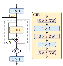
- Rank-Guided Block Design – To address redundant computation, YOLOv10 evaluates the intrinsic rank of each network stage. Less informative layers are replaced with a compact inverted block (CIB), reducing the model size without degrading accuracy.
Accuracy-Driven Model Enhancements
YOLOv10 also introduces novel accuracy-enhancing techniques to improve detection performance:
- Large-Kernel Convolution – Large-kernel depthwise convolutions increase receptive field size, enhancing the model’s ability to detect fine details. In deeper network stages, in CIB, 3×3 depthwise convolutions are replaced with 7×7 convolutions, significantly improving performance, particularly for small object detection.
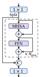
- Partial Self-Attention (PSA) – YOLOv10 introduces Partial Self-Attention (PSA), where only a portion of features are processed through multi-head self-attention (MHSA), while the rest bypass it. PSA is applied only in later stages with lower resolution, avoiding excessive overhead from the quadratic complexity of self-attention.
Training YOLOv10
Following the launch of YOLOv10, we published an in-depth article explaining the model’s architecture and functionality. To help users tailor YOLOv10 to their specific datasets, we also published “Fine-Tuning YOLOv10 Models on Custom Dataset for Kidney Stone Detection“.
YOLO11
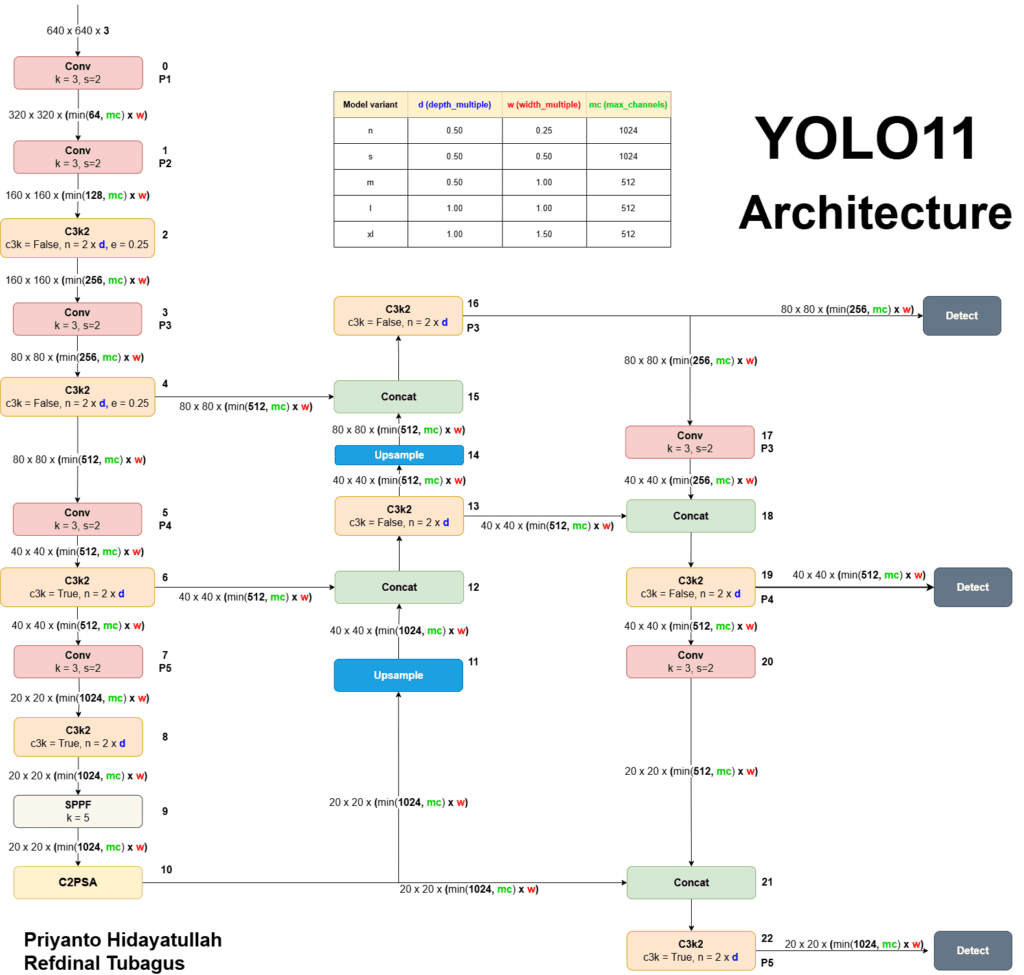
Unveiled at the YOLO Vision 2024 (YV24) Conference, this iteration builds upon the legacy of its predecessors while introducing architectural enhancements that improve feature extraction, efficiency, and multi-task adaptability.
Unlike previous versions, Ultralytics YOLO11 is designed for a broader range of computer vision tasks, including:
- Classification
- Object Detection
- Instance Segmentation
- Pose Estimation
- Oriented Object Detection (OBB)
By refining its backbone, neck, and head architecture, YOLO11 delivers improved accuracy and computational efficiency, making it a state-of-the-art model for real-time vision applications.
Architectural Enhancements in YOLO11
The YOLO series has revolutionized object detection by offering a single-stage, end-to-end trainable neural network that performs bounding box regression and classification simultaneously.
YOLO11 continues this innovation by refining its core components:
- Backbone – Extracts multi-scale features from input images.
- Neck – Aggregates and enhances features for better representation.
- Head – Generates final predictions for detection and classification.
Backbone
- Convolutional Layers – YOLO11 retains the convolutional downsampling strategy from previous versions but replaces the C2f block with a more efficient C3k2 block. improves computational efficiency by using two smaller convolutions instead of one large convolution, as seen in YOLOv8.
- SPPF and C2PSA Blocks – YOLO11 retains the Spatial Pyramid Pooling – Fast (SPPF) block, a feature extractor designed to handle objects of varying sizes effectively. A new Cross Stage Partial with Spatial Attention (C2PSA) block is introduced after SPPF, enhancing spatial attention mechanisms.
Neck
- YOLO11 replaces the C2f block in the neck with the C3k2 block improving processing speed.
- YOLO11 increases its use of spatial attention mechanisms via the C2PSA module. The inclusion of C2PSA sets YOLOv11 apart from earlier versions such as YOLOv8, which lacked this specific attention mechanism.
Head
- The C3k2 blocks are integrated into multiple processing pathways to refine feature maps efficiently at different depths.
- YOLO11 incorporates Convolution-BatchNorm-SiLU (CBS) blocks after C3k2 blocks. They help in extracting relevant features for high precision, stabilizing feature maps using Batch Normalization, and enhancing non-linearity and model performance.
Training YOLO11
Training YOLO11 involves a well-structured pipeline designed to maximize efficiency and accuracy across multiple computer vision tasks, including object tracking, instance segmentation, and pose estimation. YOLO11 achieves state-of-the-art efficiency with minimal inference latency. Fine-tuning on domain-specific datasets enhances real-world adaptability, making YOLO11 a powerful solution for autonomous systems, surveillance, and industrial AI applications.
YOLOv12
While all the previous versions in the YOLO lineup extensively uses CNN, YOLOv12 paper introduces attention mechanisms into the YOLO framework. YOLOv12 architecture consists of three key differences as compared to other YOLO variants, namely, area attention module, residual efficient layer aggregation( R-ELAN ) and some architectural improvements like using Flash attention, removing positional encoding, adjusting MLP ratio. Let’s briefly have a look at these improvements in the following sections.
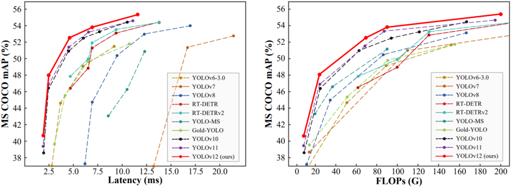
Paper Summary
Area Attention Module (A2)
YOLOv12 introduces a simple yet efficient Area Attention module (A2), which divides the feature map into segments to preserve a large receptive field while reducing the computational complexity of traditional attention mechanisms. This simple modification allows the model to retain a significant field of view while improving speed and efficiency.

Residual Efficient Layer Aggregation Networks (R-ELAN)
YOLOv12 leverages R-ELAN to address optimization challenges introduced by attention mechanisms. R-ELAN improves on the previous ELAN architecture with:
- Block-level residual connections and scaling techniques to ensure stable training.
- A redesigned feature aggregation method that improves both performance and efficiency.
Architectural Improvements
- Convolution Operators: YOLOv12 makes extensive use of convolution operations to leverage their computational efficiency, further improving performance and reducing latency.
- Flash Attention: The integration of Flash Attention addresses the memory access bottleneck of attention mechanisms, optimizing memory operations and enhancing speed.
- Removal of Positional Encoding: By eliminating positional encoding, YOLOv12 streamlines the model, making it both faster and cleaner without sacrificing performance.
- Adjusted MLP Ratio: The expansion ratio of the Multi-Layer Perceptron (MLP) is reduced from 4 to 1.2 to balance the computational load between attention and feed-forward networks, improving efficiency.
- Reduced Block Depth: By decreasing the number of stacked blocks in the architecture, YOLOv12 simplifies the optimization process and enhances inference speed.
Training YOLOv12
Shortly after the YOLOv12 paper was published, we released an introductory article that provides a short summary of the paper. Understanding how to adapt this model for use with your custom data is crucial. To assist with this, we crafted the article “Fine-Tuning YOLOv12: Comparison with YOLOv11 & Darknet-Based YOLOv7” which as the title Following this, we also published an interesting article on training custom datasets for instance segmentation with YOLOv9, and we compared the outcomes with those from YOLOv8.
Summary and Conclusion
The whole YOLO series is full of engineering innovations and breakthroughs, It offers numerous applied machine-learning ideas that can be used in specific scenarios. As Convolution Blocks are the basis for the entire YOLO series of models and as YOLO is mainly designed for edge devices, by going through all the YOLO models, one can learn different CNN optimization techniques.
- When YOLOv1 was first introduced, it was revolutionary as it pioneered the concept of a single-stage detection model. It stood out for not incorporating any region proposal mechanisms, allowing it to analyze the entire image at once and efficiently capture both global and local context.
- Later, the YOLOv2 and YOLOv3 models integrated advanced techniques that emerged at that time, such as the concept of Feature Pyramid Networks (FPN), multi-scale training, and anchor boxes.
- But, YOLOv4 was different, the authors went above and beyond to bring some ground-breaking changes to YOLO. They introduced changes in the architecture, the Darknet53, which became CSPDarknet53-PANet-SPP, techniques such as a bag of specials and freebies, Genetic Evolution algorithms, Attention modules, and so on.
- YOLOv5 brought changes that were very minimal and included most of the techniques from YOLOv4, what made YOLOv5, YOLOv5 is its Pytorch Implementation and how easy it is to train a Model using the Ultralytics.
- In YOLO-R, the authors experimented with a novel approach and worked toward evolving the model to support multi-task learning.
- But, in YOLO-X, it was again back to integrating new advances to the old YOLOv3 model, such as Anchor-free, Decoupled heads, Lable assignment and strong augmentations etc.
- In YOLOv7 and YOLOv6 authors experimented with the model architecture, YOLOv7 first brought the concept of re-parameterization in YOLO and model scaling, and YOLOv6 contributed by adding distillation and quantization techniques.
- Looking at YOLOv8 and its performance, previous models might seem over-engineered because it was built on top of YOLOv5 with minimal changes, such as replacing CSPLayer with C2f module, adding better loss functions that help the model to deal with small objects.
- YOLO-NAS was an algorithm-generated model with quantization blocks that made the model faster and more accurate.
- YOLOv10 introduced a paradigm shift in real-time object detection by eliminating Non-Maximum Suppression (NMS) through dual label assignments and a consistent matching metric, significantly reducing inference latency while maintaining high accuracy. Its efficiency-accuracy driven model design, featuring lightweight classification heads, spatial-channel decoupled downsampling, large-kernel convolutions, and Partial Self-Attention (PSA), optimized feature extraction without increasing computational overhead.
- The introduction of the C3k2 block, C2PSA attention module, and enhanced neck and head structures significantly improved feature extraction, spatial awareness, and multi-scale detection efficiency. YOLO11 extended its capabilities beyond traditional object detection, incorporating instance segmentation, pose estimation, and oriented object detection (OBB).
- The architecture of YOLOv12 is a significant step forward in real-time object detection. By incorporating Area Attention, R-ELAN, and architectural improvements such as Flash Attention, MLP ratio adjustment, and the removal of positional encoding, YOLOv12 offers a model that is faster, more efficient, and more accurate than its predecessors
💡 This article will be updated as and when new YOLO models are published.
References
[1] You Only Look Once: Unified, Real-Time Object Detection
[2] YOLO9000: Better, Faster, Stronger
[3] YOLOv3: An Incremental Improvement
[4] YOLOv4: Optimal Speed and Accuracy of Object Detection
[5] YOLOv6: A Single-Stage Object Detection Framework for Industrial Applications
[6] YOLOv7: Trainable bag-of-freebies sets new state-of-the-art for real-time object detectors
[7] YOLO-NAS by Deci Achieves SOTA Performance on Object Detection Using Neural Architecture Search
[8] A Comprehensive Review of YOLO: From YOLOv1 and Beyond
[9] YOLOv8
[10] YOLOv9
[11] YOLOv10
[12] YOLO11
[13] YOLOv12



100K+ Learners
Join Free OpenCV Bootcamp3 Hours of Learning