Semantic Segmentation using KerasCV DeepLabv3+

The KerasCV series continues with this second article. Continuing from the previous post, where we discussed Object Detection using KerasCV YOLOv8, this article discusses solving a semantic segmentation problem by fine-tuning the KerasCV DeepLabv3+ model.

DeepLabv3+ is a prevalent semantic segmentation model that finds use across various applications in image segmentation, such as medical imaging, autonomous driving, etc. 

KerasCV, too, has integrated DeepLabv3+ into its library. In this blog post, we shall extensively discuss how to leverage DeepLabv3+ and fine-tune it on our custom data. Specifically, we will use the following ImageNet pre-trained backbones as feature extractors for fine-tuning DeepLabv3+:

• ResNet50_V2
• EfficientNetv2_small

Finally, we will also compare the results across these models.

1. The Satellite Water Bodies Semantic Segmentation Dataset
   1. Pixel Differences and Mislabeled Annotations
   2. Presence of White Pixels at Boundaries of Ground Truth Masks
   3. Irrelevant Image Samples and Masks
2. Dataset Preparation for Semantic Segmentation through KerasCV
   1. Download Image Data and Ground Truth Annotations
   2. Hyper-parameter Configurations for KerasCV DeepLabv3+
   3. Dataset Preparation for Semantic Segmentation
3. Ground Truth Visualizations for Semantic Segmentation through KerasCV
4. Data Augmentation for KerasCV DeepLabv3+ Training Pipeline
5. The KerasCV DeepLabv3+ Model
   1. Model Callbacks for KerasCV DeepLabv3+
6. Evaluation Metrics
7. Training KerasCV DeepLabv3+ on the Satellite Images of Water Bodies Dataset
8. Predictions Visualization from KerasCV DeepLabv3+
9. Summary and Conclusion
10. References

The Satellite Water Bodies Semantic Segmentation Dataset

We will fine-tune our DeepLabv3 model on satellite images of waterbodies. To give a brief context on the dataset, it consists of images captured by the Sentinel-2 Satellite. Each image comes with a binary mask where white represents water and black represents the background. The masks were generated by calculating the NWDI (Normalized Water Difference Index), which is frequently used to detect and measure vegetation in satellite images, but a greater threshold was used to detect water bodies.

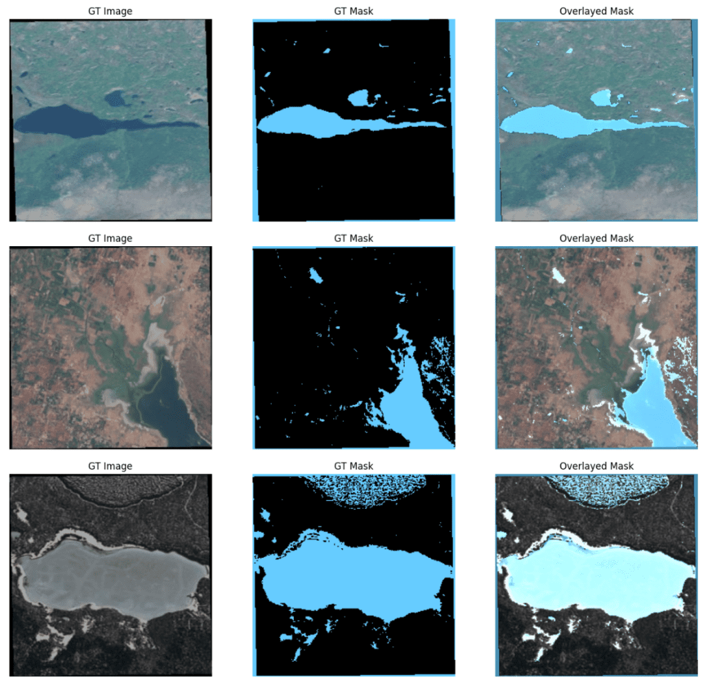
Let’s take a look at a few samples.

There are a total of 2841 samples. We will choose a 95-5 split for the train and validation splits. However, before we proceed with the data preparation, there are a few issues with the data worth mentioning.

Pixel Differences and Mislabeled Annotations

Although we have mentioned that the dataset contains binary masks as the ground truth labels, they are not genuinely binary because there are pixels that are not entirely 0 or 255. There are quite a few gray pixels in the masks. The issue can be resolved through image thresholding. Specifically, we will threshold all pixel values greater than 200 to 255 and 0 below the threshold, which essentially leaves us with precisely two classes for the labels:

• Class 0: Background
• Class 1: Water bodies (pixel values being 255).

We can also perform further morphological transformations to reduce the noise, but we shall stick to thresholding for now.

Even after thresholding, there are some mislabelled annotations, as shown below.

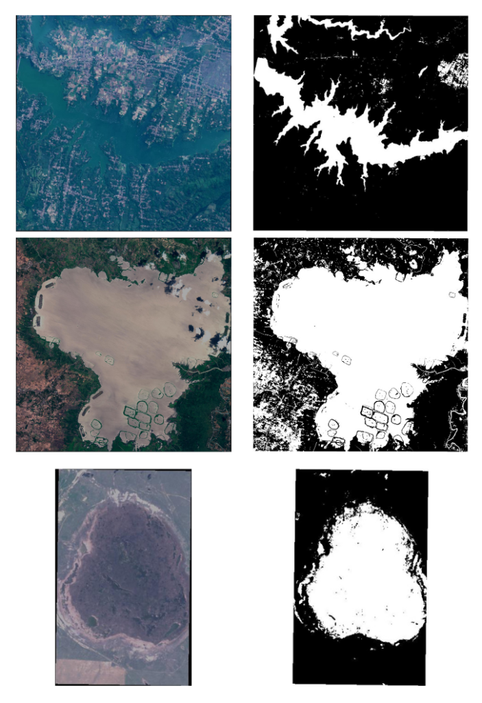
In the first two images and their corresponding masks, you can see that the buildings and some land cover are labeled as water bodies, which is incorrect. Similarly, in the second image, most of the patch of land is labeled as waterbodies. These anomalies significantly hamper model learning; however, we will keep these samples and observe how our model performs.

Presence of White Pixels at Boundaries of Ground Truth Masks

The samples below depict the boundaries of the masks labeled as waterbodies (having pixel values of 255), as shown below.

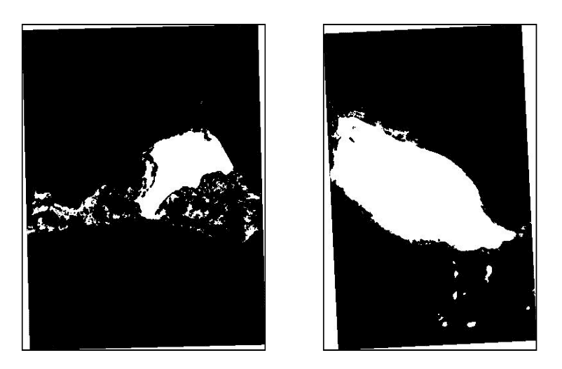
Both of the masks consist of white pixels at the edges, inadvertently labeled as water bodies, affecting model learning.

Irrelevant Image Samples and Masks

So far, we have discussed anomalies in the dataset where there were partial mislabeled annotations. However, a few samples in the dataset are completely misannotated. The image samples and their corresponding masks are shown below.

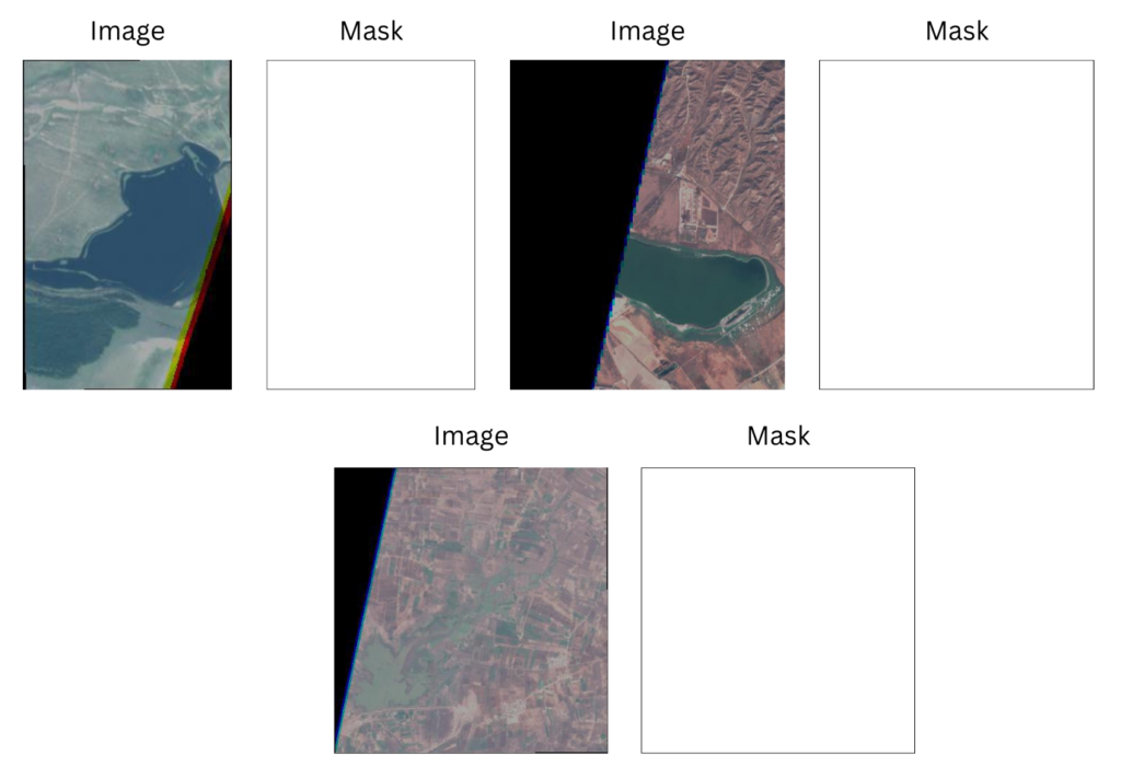
As you can observe, the entire ground truth masks across all these samples are white, indicating the presence of water bodies. Ideally, such samples should be omitted during data preparation.

 From these discussions, it is evident that real-world datasets are frequently not clean. This could significantly impact model learning during training. Hence, cleaning the data before it is passed to the neural network model is imperative.

Click here to download the source code to this post

Dataset Preparation for Semantic Segmentation through KerasCV

Before we start with the data preparation, we need to have keras_cv installed first. KerasCV contains modular computer vision components that work natively with TensorFlow, JAX, and PyTorch. It allows seamless customization of models and other training pipelines across major computer vision domains, such as classification, object detection, semantic segmentation, etc.  Use the following command to install keras_cv.

!pip install -q git+https://github.com/keras-team/keras-cv.git --upgrade

Once installed, we shall import the following dependencies for the training pipeline.

import os
import requests
from zipfile import ZipFile
import glob
from dataclasses import dataclass

import random
import numpy as np
import cv2

import tensorflow as tf
import keras_cv

import matplotlib.pyplot as plt

The next step involves maintaining the appropriate seeds for reproducibility.

def system_config(SEED_VALUE):
    # Set python `random` seed.
    # Set `numpy` seed
    # Set `tensorflow` seed.
    random.seed(SEED_VALUE)
    tf.keras.utils.set_random_seed(SEED_VALUE)
    os.environ["CUDA_VISIBLE_DEVICES"] = '0'
    os.environ['TF_CUDNN_DETERMINISTIC'] = '1'     
    os.environ['TF_USE_CUDNN'] = "true"

system_config(SEED_VALUE=42)

Download Image Data and Ground Truth Annotations

Begin by downloading the images and the ground truth masks. The download_and_unzip utility downloads and extracts the required data.

def download_and_unzip(url, save_path):

    print("Downloading and extracting assets...", end="")
    file = requests.get(url)
    open(save_path, "wb").write(file.content)

    try:
        # Extract tarfile.
        if save_path.endswith(".zip"):
            with ZipFile(save_path) as zip:
                zip.extractall(os.path.split(save_path)[0])

        print("Done")
    except:
        print("Invalid file")

In order to download this, the dataset URL has to be specified. The required data will be extracted once the download has been completed.

DATASET_URL = r"https://www.dropbox.com/scl/fi/9k8t9619b4x0hegued5c5/Water-Bodies-Dataset.zip?rlkey=tjgepcai6t74yynmx7tqsm7af&dl=1"
DATASET_DIR = "Water-Bodies-Dataset"
DATASET_ZIP_PATH = os.path.join(os.getcwd(), f"{DATASET_DIR}.zip")

# Download if dataset does not exists.
if not os.path.exists(DATASET_DIR):
    download_and_unzip(DATASET_URL, DATASET_ZIP_PATH)
    os.remove(DATASET_ZIP_PATH)

Once extracted, the directory will have the following structure.

Water-Bodies-Dataset/
├── Images
│   ├── water_body_1.jpg
│   ├── water_body_2.jpg
│   └── … (2841 files)
└── Masks
   ├── water_body_1.jpg
   ├── water_body_2.jpg
   └── … (2841 files)

Hyper-parameter Configurations for KerasCV DeepLabv3+

Next, we will define the various hyper-parameter settings that will be used throughout our training pipeline.

Data Configuration for KerasCV DeepLabv3

The DatasetConfig class takes in the various hyperparameters related to the data, such as the image size and batch size to be used while training, the number of classes being used, and the various augmentation factors such as random brightness, random contrast, etc.

@dataclass(frozen=True)
class DatasetConfig:
    IMAGE_SIZE:        tuple = (256, 256)
    BATCH_SIZE:          int = 16
    NUM_CLASSES:         int = 2
    BRIGHTNESS_FACTOR: float = 0.2
    CONTRAST_FACTOR:   float = 0.2

Training Configuration for KerasCV DeepLabv3

The training hyper-parameters, such as model backbone, the number of epochs, learning rate, etc., are handled by the TrainingConfig class.

@dataclass(frozen=True)
class TrainingConfig:
    MODEL:           str = "resnet50_v2_imagenet"
    EPOCHS:          int = 35
    LEARNING_RATE: float = 1e-4
    CKPT_DIR:        str = os.path.join("checkpoints_"+"_".join(MODEL.split("_")[:2]), 
                                        "deeplabv3_plus_"+"_".join(MODEL.split("_")[:2])+".h5")
    LOGS_DIR:        str = "logs_"+"_".join(MODEL.split("_")[:2])

For the EfficientNetv2_s backbone, we can specify “efficientnetv2_s_imagenet” as the feature extractor.

Dataset Preparation for Semantic Segmentation

TensorFlow’s tf.data API will be used, which enables us to build complex pipelines using simple, reusable code components. It allows us to handle large amounts of data, perform complex transformations, manage data across multiple formats, etc.

We proceed by specifying the image file paths and the ground truth masks. Next, we randomly shuffle these paths to avoid any unnecessary bias during training.

data_images = glob.glob(os.path.join(DATASET_DIR, "Images", "*.jpg"))
data_masks = glob.glob(os.path.join(DATASET_DIR, "Masks", "*.jpg"))

# Shuffle the data paths before data preparation.
zipped_data = list(zip(data_images, data_masks))
random.shuffle(zipped_data)
data_images, data_masks = zip(*zipped_data)
data_images = list(data_images)
data_masks = list(data_masks)

Creating tensor slices will combine the images and mask file paths to a TensorFlow Dataset. This is achieved using the tf.data.Dataset.from_tensor_slices method.

org_data = tf.data.Dataset.from_tensor_slices((data_images, data_masks))

Train and Validation Splits

Now that the images and masks are coupled into a TensorFlow dataset, we split them into training and validation paths by maintaining a 95-5 split ratio between them.

SPLIT_RATIO = 0.05
# Determine the number of validation samples
NUM_VAL = int(len(data_images) * SPLIT_RATIO)

# Split the dataset into train and validation sets
train_data = org_data.skip(NUM_VAL)
valid_data = org_data.take(NUM_VAL)

Data Loading and Mask Preprocessing

We will now load the images and masks from the Dataset created using the file paths. While loading, we will maintain a  (256, 256) image resolution for resizing the images and masks. 
We will threshold the pixel values of the masks ranging above 200 to 255; and update the pixels to 0 for values lying below 200. The final step will be to maintain the following dictionary, which maps input images with masks.

{"images": image, "segmentation_masks": mask}

The read_image_mask function loads and resizes the inputs from the file paths. Additionally, it also performs mask thresholding.

def read_image_mask(image_path, mask=False, size = data_config.IMAGE_SIZE):
    image = tf.io.read_file(image_path)

    if mask:
        image = tf.io.decode_image(image, channels=1)
        image.set_shape([None, None, 1])
        image = tf.image.resize(images=image, size=size, method = "bicubic")

        image_mask = tf.zeros_like(image)
        cond = image >=200
        updates = tf.ones_like(image[cond])
        image_mask = tf.tensor_scatter_nd_update(image_mask, tf.where(cond), updates)
        image = tf.cast(image_mask, tf.uint8)

    else:
        image = tf.io.decode_image(image, channels=3)
        image.set_shape([None, None, 3])
        image = tf.image.resize(images=image, size=size, method = "bicubic")
        image = tf.cast(tf.clip_by_value(image, 0., 255.), tf.float32)

    return image

The load_data function uses the read_image_mask utility function to perform appropriate pre-processing given the input image and mask paths and return the appropriate dictionary mappings.

def load_data(image_list, mask_list):
    image = read_image_mask(image_list)
    mask  = read_image_mask(mask_list, mask=True)
    return {"images":image, "segmentation_masks":mask}

We will now create the training and validation datasets.

train_ds = train_data.map(load_data, num_parallel_calls=tf.data.AUTOTUNE)
valid_ds = valid_data.map(load_data, num_parallel_calls=tf.data.AUTOTUNE)

The unpackage_inputs is a utility function that is used to unpack the inputs from the dictionary format to a tuple (images, segmentation_masks). This will be used later for visualizing the images, segmentation masks, and model predictions.

def unpackage_inputs(inputs):
    images = inputs["images"]
    segmentation_masks = inputs["segmentation_masks"]
    return images, segmentation_masks

Ground Truth Visualizations for Semantic Segmentation through KerasCV

The color mapping dictionary id2color below defines the mapping between class IDs and RGB colors for visualizations.

id2color = {
    0: (0,  0,    0),    # Background
    1: (102, 204, 255),  # Waterbodies
 }

The utility function num_to_rgb will convert a single-channel mask to an RGB representation for visualization purposes. Each class ID in the single-channel mask will be converted to a different color according to the id2color dictionary mapping.

def num_to_rgb(num_arr, color_map=id2color):
    
    # single_layer = np.squeeze(num_arr)
    output = np.zeros(num_arr.shape[:2]+(3,))
    
    for k in color_map.keys():
        output[num_arr==k] = color_map[k]
        
    return output.astype(np.uint8)

The image_overlay utility is used to overlay the RGB segmented mask on top of the corresponding RGB image.

# Function to overlay a segmentation map on top of an RGB image.
def image_overlay(image, segmented_image):

    alpha = 1.0 # Transparency for the original image.
    beta  = 0.7 # Transparency for the segmentation map.
    gamma = 0.0 # Scalar added to each sum.

    image = image.astype(np.uint8)

    segmented_image = cv2.cvtColor(segmented_image, cv2.COLOR_RGB2BGR)

    image = cv2.cvtColor(image, cv2.COLOR_RGB2BGR)

    image = cv2.addWeighted(image, alpha, segmented_image, beta, gamma, image)
    image = cv2.cvtColor(image, cv2.COLOR_BGR2RGB)

    return image

The convenience function display_image_and_mask will display the original image, the ground truth mask, and the overlayed ground truth mask on the original image. 

Besides, it also offers to plot predicted segmentation mask and have it overlayed on the input image. Note that an optional argument allows you to control whether the ground truth mask is displayed as a grayscale or color image.

def display_image_and_mask(data_list, title_list, figsize, color_mask=False, color_map=id2color):
    
    # Create RGB segmentation map from grayscale segmentation map.
    rgb_gt_mask = num_to_rgb(data_list[1], color_map=color_map)
    mask_to_overlay = rgb_gt_mask

    if len(data_list)==3:
        rgb_pred_mask = num_to_rgb(data_list[-1], color_map=color_map)
        mask_to_overlay = rgb_pred_mask
        
    # Create the overlayed image.
    overlayed_image = image_overlay(data_list[0], mask_to_overlay)
    
    data_list.append(overlayed_image)

    fig, axes = plt.subplots(nrows=1, ncols=len(data_list), figsize=figsize)
    
    for idx, axis in enumerate(axes.flat):
        axis.set_title(title_list[idx])
        if title_list[idx] == "GT Mask":
            if color_mask:
                axis.imshow(rgb_gt_mask)
            else:
                axis.imshow(data_list[1], cmap="gray")

        elif title_list[idx] == "Pred Mask":
            if color_mask:
                axis.imshow(rgb_pred_mask)
            else:
                axis.imshow(data_list[-1], cmap="gray")
            
        else:
            axis.imshow(data_list[idx])
            
        axis.axis('off')
        
    plt.show()

Let us now plot a few ground truth samples.

plot_train_ds = train_ds.map(unpackage_inputs).batch(3)
image_batch, mask_batch = next(iter(plot_train_ds.take(1)))

titles = ["GT Image", "GT Mask", "Overlayed Mask"]

for image, gt_mask in zip(image_batch, mask_batch):

    gt_mask = tf.squeeze(gt_mask, axis=-1).numpy()
    display_image_and_mask([image.numpy().astype(np.uint8), gt_mask], 
                           title_list=titles,
                           figsize=(16,6),
                           color_mask=True)

Data Augmentation for KerasCV DeepLabv3+ Training Pipeline

KerasCV’s RandomFlip, RandomBrightness, and RandomContrast will be used to apply image augmentation. Applying augmentations to the validation data should be avoided.

Note: Horizontal Flip is applied by default with a probability factor of 0.5. Vertical or both horizontal and vertical flips can also be applied by specifying the mode. The probability factor is maintained using the rate argument.

augment_fn = tf.keras.Sequential(
    [
        keras_cv.layers.RandomFlip(),
        keras_cv.layers.RandomBrightness(factor=data_config.BRIGHTNESS_FACTOR,
                                         value_range=(0, 255)),
        keras_cv.layers.RandomContrast(factor=data_config.CONTRAST_FACTOR,
                                       value_range=(0, 255)),
    ]
)

Using the batch size defined in the TrainingConfig class, we create the final training and validation datasets. The training set is also shuffled and mapped with the augment_fn.

train_dataset = (
                train_ds.shuffle(data_config.BATCH_SIZE)
                .map(augment_fn, num_parallel_calls=tf.data.AUTOTUNE)
                .batch(data_config.BATCH_SIZE)
                .map(unpackage_inputs)
                .prefetch(buffer_size=tf.data.AUTOTUNE)
)

valid_dataset = (
                valid_ds.batch(data_config.BATCH_SIZE)
                .map(unpackage_inputs)
                .prefetch(buffer_size=tf.data.AUTOTUNE)
)

The KerasCV DeepLabv3+ Model

Read this article to understand the DeepLabv3+ model architecture thoroughly.

We will create the DeepLabv3 model using pre-trained ImageNet classification backbones precisely:

• ResNet50_v2
• EfficientNetv2_small

The DeepLab segmentation head will be initialized with random weights.

The following code snippet creates the deeplabv3_plus model using the ResNet50_v2 backbone.

backbone = keras_cv.models.ResNet50V2Backbone.from_preset(preset = train_config.MODEL,
                                                          input_shape=data_config.IMAGE_SIZE+(3,),
                                                          load_weights = True)
model = keras_cv.models.segmentation.DeepLabV3Plus(
        num_classes=data_config.NUM_CLASSES, backbone=backbone,
    )

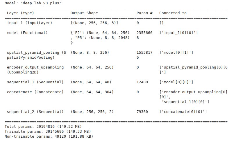
The built model contains approximately 39M parameters, as vindicated by the model summary.

We can load the appropriate weights to build the model using the EfficientNetv2 backbone.

backbone = keras_cv.models.EfficientNetV2Backbone.from_preset(preset = train_config.MODEL,
                                                          input_shape=data_config.IMAGE_SIZE+(3,),
                                                          load_weights = True)
model = keras_cv.models.segmentation.DeepLabV3Plus(
        num_classes=data_config.NUM_CLASSES, backbone=backbone,
    )

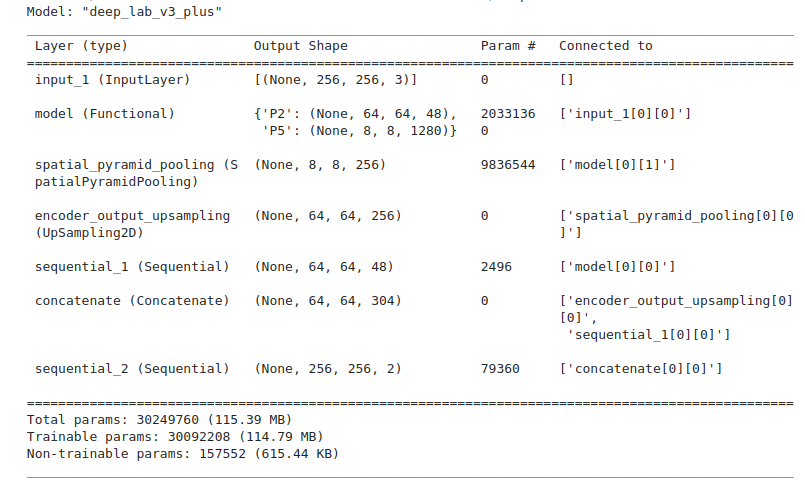
It contains around 30M parameters, as observed from the summary.

Model Callbacks for KerasCV DeepLabv3

We will use the Tensorboard and ModelCheckpoint callbacks to log the losses and metrics and save the model weights. The weights will be saved on the best validation mIoU score. 

The get_callbacks utility defines the callbacks during model training.

def get_callbacks(
    train_config,
    monitor="val_mean_iou",
    mode="max",
    save_weights_only=True,
    save_best_only=True,
):

    # Initialize tensorboard callback for logging.
    tensorboard_callback = tf.keras.callbacks.TensorBoard(
        log_dir=train_config.LOGS_DIR,
        histogram_freq=20,
        write_graph=False,
        update_freq="epoch",
    )


    # Update file path if saving best model weights.
    if save_weights_only:
        checkpoint_filepath = train_config.CKPT_DIR

    model_checkpoint_callback = tf.keras.callbacks.ModelCheckpoint(
        filepath=checkpoint_filepath,
        save_weights_only=save_weights_only,
        monitor=monitor,
        mode=mode,
        save_best_only=save_best_only,
        verbose=1,
    )

    return [tensorboard_callback, model_checkpoint_callback]

Evaluation Metrics

Intersection over Union (IoU) is a metric often used in segmentation problems to assess the model’s accuracy. It provides a more intuitive basis for accuracy that is not biased by the (unbalanced) percentage of pixels from any particular class. Given two segmentation masks, `A` and `B`, the IoU is defined as follows:

When multiple classes and inferences exist, we assess the model’s performance by computing the mean IoU. 

The function mean_iou below computes the mean IoU that only considers the classes that are present in the ground truth mask or the predicted segmentation map (sometimes referred to as classwise mean IoU). This computation better represents the metric since it only considers the relevant classes. We use this metric computation for mean IoU.

def mean_iou(y_true, y_pred):

    # Get total number of classes from model output.
    num_classes = y_pred.shape[-1]

    y_true = tf.squeeze(y_true, axis=-1)

    y_true = tf.one_hot(tf.cast(y_true, tf.int32), num_classes, axis=-1)
    y_pred = tf.one_hot(tf.math.argmax(y_pred, axis=-1), num_classes, axis=-1)

    # Intersection: |G ∩ P|. Shape: (batch_size, num_classes)
    intersection = tf.math.reduce_sum(y_true * y_pred, axis=(1, 2))

    # Total Sum: |G| + |P|. Shape: (batch_size, num_classes)
    total = tf.math.reduce_sum(y_true, axis=(1, 2)) + tf.math.reduce_sum(y_pred, axis=(1, 2))

    union = total - intersection

    is_class_present =  tf.cast(tf.math.not_equal(total, 0), dtype=tf.float32)
    num_classes_present = tf.math.reduce_sum(is_class_present, axis=1)

    iou = tf.math.divide_no_nan(intersection, union)
    iou = tf.math.reduce_sum(iou, axis=1) / num_classes_present

    # Compute the mean across the batch axis. Shape: Scalar
    mean_iou = tf.math.reduce_mean(iou)

    return mean_iou

The next step is to define the loss function and optimizer and finally compile the model.

# Build model.

# Get callbacks.
callbacks = get_callbacks(train_config)
# Define Loss.
loss_fn = tf.keras.losses.SparseCategoricalCrossentropy(from_logits=False)
# Compile model.
model.compile(
    optimizer=tf.keras.optimizers.Adam(train_config.LEARNING_RATE),
    loss=loss_fn,
    metrics=["accuracy", mean_iou],
)

Since we are dealing with two classes, we have used the SparseCategoricalCrossentropy loss function.

Note: The parameter from_logits=False has been used since the softmax is already implemented as the final activation layer inside the network.

Training KerasCV DeepLabv3+ on the Satellite Images of Water Bodies Dataset

We are now ready to train the model. We initiate training by calling the model.fit() function on the already configured data.

# Train the model, doing validation at the end of each epoch.
history = model.fit(
    train_dataset,
    epochs=train_config.EPOCHS,
    validation_data=valid_dataset,
    callbacks=callbacks
)

The plots show the logs for the DeepLabv3+ model with ResNet50_v2 backbone.

We achieved a mean pixel accuracy score of 0.9422 and a mean IoU score of 0.8299.

The orange curve represents the training logs, while the blue ones represent the validation logs.

You can take a closer look at the tensorboard logs for the ResNet50_V2 model.

The plot below shows the logs for the DeepLabv3+ model with EfficientNetv2_small backbone.

We achieved a mean pixel accuracy score of 0.9399 and a mean IoU score of 0.8324.

This is great, considering EfficientNetv2_small has comparatively fewer training parameters than ResNet50_v2.

The tensorboard logs for the EfficientNetV2_small model have also been uploaded.

From the training logs above, it can be observed that the validation plots are smoother for EfficientNet_V2_small compared to those of ResNet50_V2.

Predictions Visualization from KerasCV DeepLabv3

Now that we have performed training let us visualize a few sample predictions.

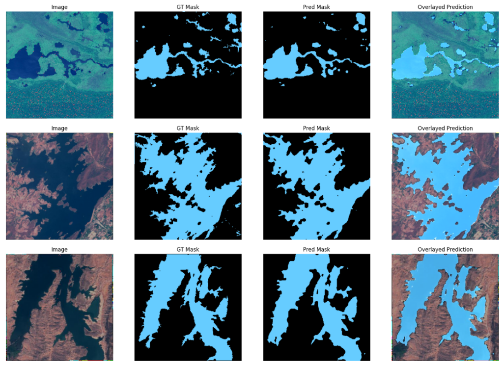
The inference plots ten prediction samples from the validation data using the fine-tuned model.

def inference(model, dataset, samples_to_plot):

    num_batches_to_process = 2
    count = 0
    stop_plot = False

    titles = ["Image", "GT Mask", "Pred Mask", "Overlayed Prediction"]

    for idx, data in enumerate(dataset):

        if stop_plot:
            break

        batch_img, batch_mask = data[0], data[1]
        batch_pred = (model.predict(batch_img)).astype('float32')
        batch_pred = batch_pred.argmax(axis=-1)
        
        batch_img  = batch_img.numpy().astype('uint8')
        batch_mask = batch_mask.numpy().squeeze(axis=-1)

        for image, mask, pred in zip(batch_img, batch_mask, batch_pred):
            count+=1
            display_image_and_mask([image, mask, pred],
                                  title_list=titles,
                                   figsize=(20,8),
                                   color_mask=True)
            if count >= samples_to_plot:
                stop_plot=True
                break
            

Sample predictions using the ResNet50_v2 backbone.

Sample predictions using the EfficientNetv2_small backbone.

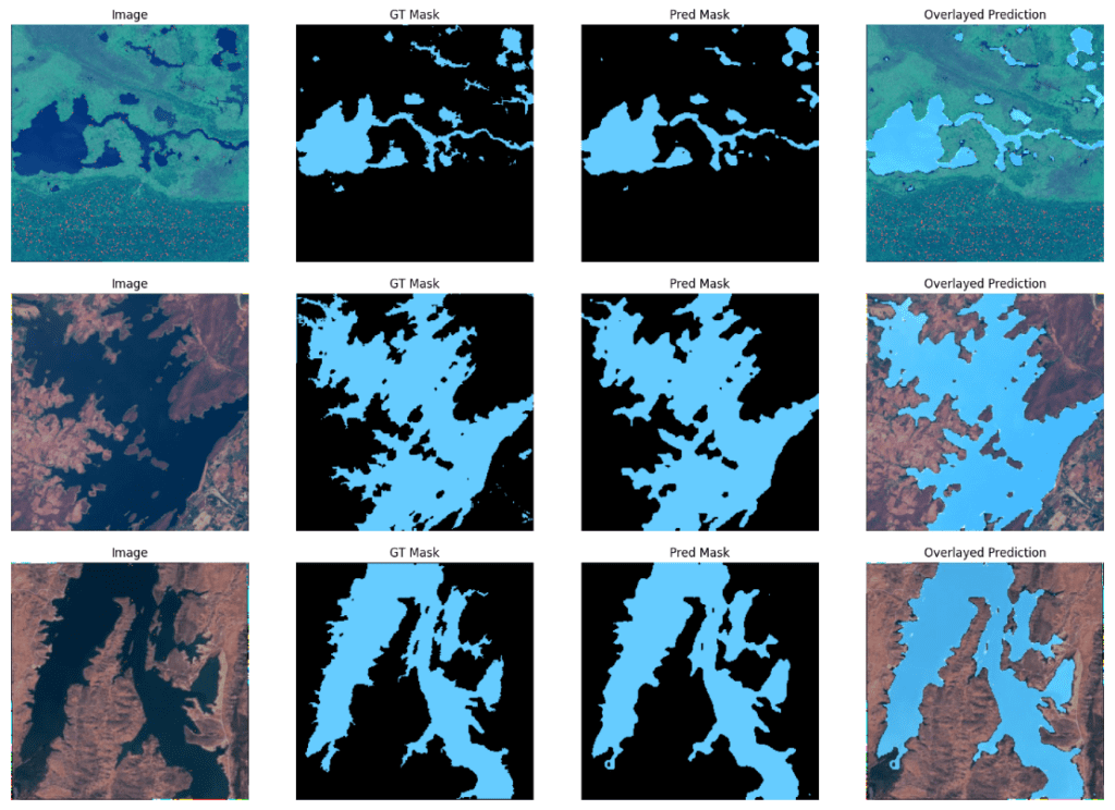
We can observe that although DeepLabv3+ with EfficientNet_v2_small has a slightly higher mIOU score, there aren’t any significant differences in the visualizations between the two.

Both models perform really well across these samples.

Now, let’s observe a couple of hard example instances from the ResNet50v2 model.

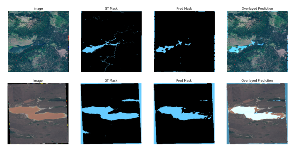
You can see that for both images, the model predicts the boundary pixels of the input image as water bodies. However, even their corresponding ground truth masks are mislabeled; consequently, it contributed to the model misclassifying the boundary pixels.

It can be deduced that the model performs decently in these instances even though they are relatively difficult examples.

The model performance can be enhanced by addressing the data anomalies described earlier. Complex data augmentation transformations can also be added to improve the model performance.

Summary and Conclusion

To wrap up, we’ve covered various aspects in this article. We started by introducing DeepLabv3+ as a part of the KerasCV library. Addressing anomalies in our dataset was a key focus, and we demonstrated how to eliminate them. We prepared the dataset, after which we fine-tuned it. We also showcased how to implement different backbones on top of the DeepLabv3 segmentation head and compared the results across the different backbones. We trust that you have found this article interesting and informative. We eagerly await your thoughts and comments below!

References

1. Satellite Image of Water Bodies
2. KerasCV – Image Segmentation using UNet
3. KerasCV Repository
4. KerasCV Pre-trained Models and Presets
5. KerasCV Augmentation Layers