GradCAM – Enhancing Neural Network Interpretability in the Realm of Explainable AI

With millions of trainable parameters, neural networks have long been considered black boxes. They can produce stunning results, and we often accept the output with very little understanding as to why the model makes the predictions that it does. In some cases, models can learn unintended correlations and produce “correct” results unrelated to the intended task. GradCAM, an acronym for Gradient-weighted Class Activation Mapping, is a significant breakthrough in computer vision and neural network interpretability. As AI and machine learning systems, particularly Convolutional Neural Networks (CNNs), become increasingly integrated into various aspects of technology and daily life, understanding their decision-making processes has become paramount. This is where GradCAM steps in as a pivotal tool.

We will begin the article by fine-tuning a popular classification model, specifically, EfficienNetV2 small on the Brain MRI dataset for classifying four categories of brain tumors evident in the scans. Once fine-tuned, we will discuss the underlying principles for implementing GradCAM to demonstrate model interpretability.

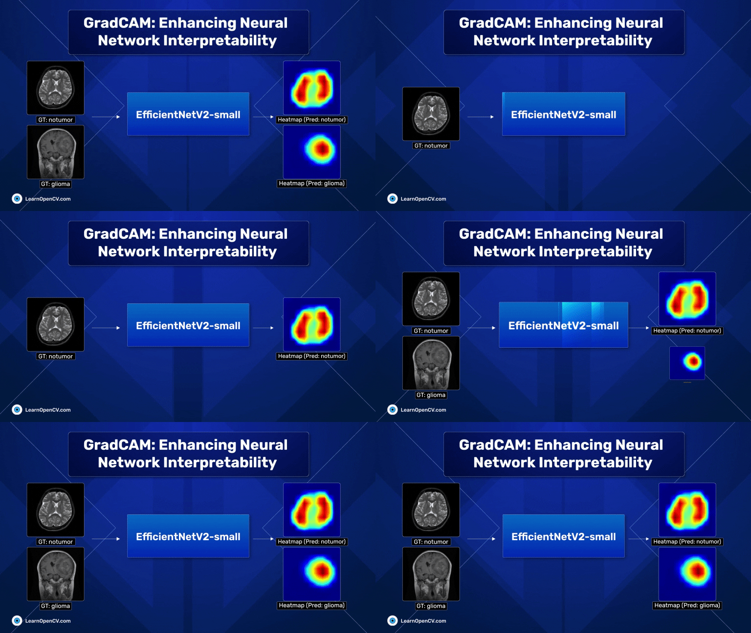
Scroll through the GradCAM results on the Brain MRI data for a quick look.

1. The Brain MRI Scan Data for Brain Tumor Classification
2. Pipeline for Implementing GradCAM on the Brain MRI Data
3. Managing Installation Packages and Imports
4. Hyperparameter Configuration for Training and Fine-tuning
5. Data Preparation for Fine-tuning the Brain MRI Data
6. Fine-Tuning EfficientNet V2 on Brain MRI Data
7. Creating Custom LightningModule Class
8. Fine-tuning and Training
9. Model Evaluation and Inference
10. Class Activation Mapping (CAM)
11. Introduction to GradCAM
12. GradCAM Visualizations
13. Summary and Conclusion
14. References

The Brain MRI Scan Data for Brain Tumor Classification

The dataset consists of 1311 Brain MRI scans, primarily curated for brain tumor classification. The dataset deals explicitly with four categories of brain tumors, namely:

• Glioma (300 samples)
• Meningioma (306 samples)
• No tumor (405 samples)
• Pituitary (300 samples)

The dataset is more or less balanced, with a slight excess of non-tumor sample instances.

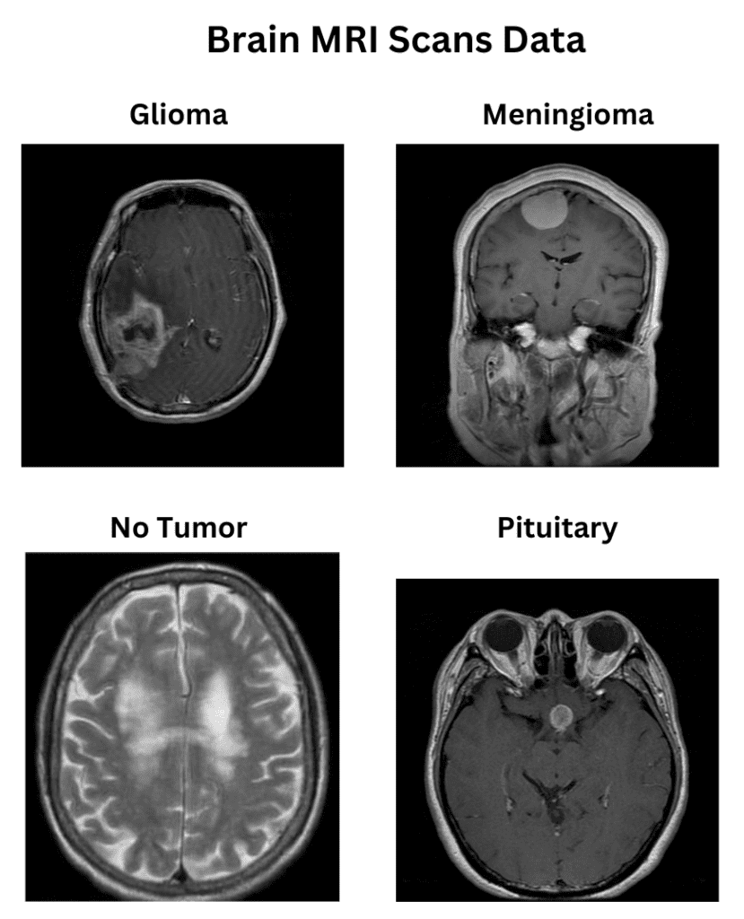
The dataset is divided into the corresponding classes as separate directories. The directory structure is as follows:

data
├── glioma
│   ├── Te-gl_0010.jpg
│   ├── Te-gl_0011.jpg
│   └── ...
├── meningioma
│   ├── Te-me_0010.jpg
│   ├── Te-me_0011.jpg
│   └── ...
├── notumor
│   ├── Te-no_0010.jpg
│   ├── Te-no_0011.jpg
│   └── ...
└── pituitary
    ├── Te-pi_0010.jpg
    ├── Te-pi_0011.jpg
    └── ...

The directory structure above makes it convenient to use Torchvision’s ImageFolder dataset, which can be subsequently split to train and validation sets. We have maintained an 80-20 split for the training and validation data.

Pipeline for Implementing GradCAM on the Brain MRI Data 

We shall implement a two-fold pipeline for our final GradCam implementation. This primarily involves the following steps:

• A pre-trained ImageNet classification model is fine-tuned on the given dataset.
• Implementation of GradCam on the fine-tuned model during inference.

For the fine-tuning process, we shall use the EfficientNetv2-small model. The training is carried out on images resized to 384×384 before normalizing them with the ImageNet mean and standard deviation (mean = [0.485, 0.456, 0.406], std = [0.229, 0.224, 0.225]).

You can check the architectural details of EfficientNet through our article. 

The feature extractor of the model is frozen except for the final two feature blocks. The primary reason for following this approach is that the features learned by the initial layers’ weights already have decent generalizable features; consequently, we can keep them the same.

One important point to note is that since we are creating the train and validation splits on the fly, we need to keep track of the validation files, which will be used for inference while implementing GradCam. The filenames of the validation images and their corresponding ground truth labels are maintained in the validation_samples.csv file created while implementing the Dataset class.

We will also leverage the power of lightning API, which enables us to implement the training pipeline within optimized lines of code.

In the following sections, we will examine the pipeline in more detail.

Managing Installation Packages and Imports

To expedite the training process in PyTorch, we shall use the PyTorch Lightning API, which enables us to write hassle-free optimized code with maximal flexibility and scale our projects in production.

We shall also require torchmetrics to evaluate our model as training progresses. Torchmetrics consists of various evaluation metrics across regression, classification, detection, information retrieval, and several other domains.

We begin by installing these packages alongside torchinfo for printing the model summary.

!pip install -q lightning torchmetrics torchinfo

Once installed, we will import the following dependencies.

import os
import numpy as np
import csv

import torch
import torch.nn as nn
import torch.nn.functional as F
from torch import optim
from torch.utils.data import Dataset, DataLoader, random_split
from torchvision import transforms as T, datasets, models
from torchvision.models import EfficientNet_V2_S_Weights

import lightning.pytorch as pl
from torchmetrics import MeanMetric
from torchmetrics.classification import MulticlassAccuracy, ConfusionMatrix
from lightning.pytorch.loggers import TensorBoardLogger
from lightning.pytorch.callbacks import ModelCheckpoint
from torchinfo import summary

from dataclasses import dataclass

import matplotlib.pyplot as plt

from PIL import Image

Click here to download the source code to this post

Hyperparameter Configuration for Training and Fine-tuning

We shall maintain a set of hyperparameters throughout the pipeline. This starts with the data parameters, such as batch size, number of workers, the train-validation split, etc., and the training parameters, such as the number of epochs, choice of the optimizer, learning rate, etc.

The DataConfiguration class consists of the following data hyperparameters:

• data_root : The root directory containing the image data.
• num_workers: the number of workers to enhance parallel batch data loading through sub-processes. 
• batch_size: the batch size to use
• train_val_split: the training and validation split ratios
• num_classes: the number of classes in the data

@dataclass(frozen=True)
class DataConfiguration:
    data_root: str = f"data"
    num_workers: int = 4
    batch_size: int = 32
    train_val_split: tuple = (0.8, 0.2)
    num_classes = 4

The TrainingConfiguration class consists of the following training hyperparameters:

• epochs: the number of epochs to train
• blocks_to_ft: the number of blocks in the feature extractor to fine-tune 
• optimizer: the optimizer (using Adam as the default optimizer)
• lr : the initial learning rate
• weight_decay: the weight decay used as the L2 norm
• train_logs: the directory to save the training logs such as model checkpoints, tensorboard event files, etc
• precision: 16-bit mixed precision training for computational speedup

@dataclass(frozen=True)
class TrainingConfiguration:
    '''
    Describes the configuration of the training process
    '''
    epochs: int = 25
    blocks_to_ft: int = 2
    optimizer: str = "Adam"
    lr: float = 1e-4  # initial learning rate for lr scheduler
    weight_decay: float = 5e-4
    train_logs: str = "EffNet-FT-Logs"
    precision: str = "16-mixed"

Data Preparation for Fine-tuning the Brain MRI Data

The PyTorch Lightning API offers to write our custom LightningDataModule class that encapsulates data processing steps such as:

• Data loading 
• Creating training, validation, and test sets
• Apply appropriate transformations, including data augmentations
• Creating corresponding data loaders

However, before implementing our custom DataModule class, we must implement a few additional steps.

Download and Extract the Dataset

The download_and_unzip utility downloads the data from the specified URL and extracts it from the downloaded zip file.

def download_and_unzip(url, save_path):

    print("Downloading and extracting assets...", end="")
    file = requests.get(url)
    open(save_path, "wb").write(file.content)

    try:
        # Extract zipfile.
        if save_path.endswith(".zip"):
            with ZipFile(save_path) as zip:
                zip.extractall(os.path.split(save_path)[0])

        print("Done")
    except:
        print("Invalid file")

Image Preprocessing Transformations

Before training our data, the pre-trained model expects the images to be of a specified type and shape. The img_preprocess_transforms utility applies the required transformations to the input PIL image so that it can forward propagated through the model.

This set of transformations includes the following steps:

• Resizing the image data to a fixed image resolution (for EfficientNetV2-small, the resize dimensions are 384×384)
• Rescaling the data in the range [0, 1] given an unsigned int-8 image
• Normalizing the data across the ImageNet mean and standard deviation

def img_preprocess_transforms():
    preprocess = EfficientNet_V2_S_Weights.IMAGENET1K_V1.transforms()
    return preprocess

Applying Appropriate Transforms for Training and Validation Data

Once we split the data into the corresponding train and validation data, we need to ensure the appropriate transforms are being applied across the data sets. For instance, data augmentation needs to be applied only to the training data, apart from pre-processing transforms, which are applied to both the training and validation data.

The BrainMRITransforms Dataset class accepts the required dataset (training or validation), its corresponding transforms, and the class name-to-id mapping. It returns the transformed image and class label through the __getitem__ class method.

class BrainMRITransforms(Dataset):
    def __init__(self, dataset, transforms, classes, class_to_idx):
        self.dataset = dataset
        self.transforms = transforms
        self.classes = classes
        self.class_to_idx = class_to_idx
        
    def __getitem__(self, idx):
        image, target = self.dataset[idx]
        
        if self.transforms:
            image = self.transforms(image)
            
        return image, target
    
    def __len__(self):
        return len(self.dataset)

Creating the Custom DataModule Class to Handle Data

Once the helper utilities and classes are ready, we can create the custom DataModule class offered by the Lightning API wrapper.

The Brain_MRI_DataModule class (which inherits the pl.LightningDataModule class) consists of the following class methods:

• __init__ (): Accepts the image directory path, the train-val split, the batch size, the number of classes, and the number of workers.
  It also defines the data augmentation transformations apart from the preprocess transformations.

def __init__(self, img_dir, train_val_split, batch_size, num_workers, num_classes):
        super().__init__()
        self.img_dir = img_dir
        self.train_val_split = train_val_split        
        self.batch_size = batch_size
        self.num_workers = num_workers
        self.num_classes = num_classes

        preprocess = img_preprocess_transforms()
        
        self.train_augment = T.Compose([
                                T.RandomHorizontalFlip(),
                                T.RandomRotation(degrees=10),
                                preprocess
                            ])
        
        self.valid_augment = T.Compose([
                                preprocess,
                            ])

• prepare_data(): It calls the download_and_unzip utility to download the data.

def prepare_data(self):
        DATASET_URL = r"https://www.dropbox.com/scl/fi/8xh03beb47jbaug5sxz44/brain_mri.zip?rlkey=c05xd8dyuzz8ev5scacwcnlzt&dl=1"
        DATA_ZIP_FILE = f"brain_mri.zip"
        DATASET_DIR = self.img_dir
        DATASET_ZIP_PATH = os.path.join(os.getcwd(), f"{DATA_ZIP_FILE}.zip")
        
        # Download if dataset does not exists.
        if not os.path.exists(DATASET_DIR):
            download_and_unzip(DATASET_URL, DATASET_ZIP_PATH)
            os.remove(DATASET_ZIP_PATH)

• setup(): This is where the image data is split into the respective train and validation sets based on the split ratio. As discussed, we also need to keep track of the validation image files and their ground truth class labels. Therefore, we created the validation_samples.csv file comprising the image file paths and the class labels.

def setup(self, *args, **kwargs):
        
        image_dataset = datasets.ImageFolder(root=self.img_dir)
        mri_classes = image_dataset.classes
        cls_to_idx = image_dataset.class_to_idx
        
        train_set, val_set = random_split(image_dataset, self.train_val_split)
        
        # Create train set after split.
        self.train_dataset = BrainMRITransforms(
                                dataset = train_set,
                                transforms = self.train_augment,
                                classes = mri_classes,
                                class_to_idx = cls_to_idx
                                )

        # Create validation set after split.
        self.val_dataset = BrainMRITransforms(
                                dataset = val_set,
                                transforms = self.valid_augment,
                                classes = mri_classes,
                                class_to_idx= cls_to_idx
                                )

        # Create csv file for validation data for inference later on.
        # -----------------------------------------------------------

        csv_filename = "validation_samples.csv"
        # Fields of CSV files for creating validation samples.
        fields = ["Filename", "Target"]
        
        # Index the filenames and targets from image_dataset based on vals-split.
        val_samples = [image_dataset.samples[idx] for idx in val_set.indices]

        # Create the csv file.
        with open(csv_filename, "w", newline="") as csv_file:
            csv_writer = csv.writer(csv_file)
            csv_writer.writerow(fields)
            csv_writer.writerows(val_samples)

• train_dataloader(): creates the training dataloader.

def train_dataloader(self):
        return DataLoader(self.train_dataset,
                          batch_size = self.batch_size,
                          num_workers = self.num_workers,
                          shuffle = True,
                          pin_memory=True
                          )

• val_dataloader(): creates the validation data loader.

def val_dataloader(self):
        return DataLoader(self.val_dataset,
                          batch_size = self.batch_size,
                          num_workers = self.num_workers,
                          shuffle = False,
                          pin_memory=True
                          )

Dataset Visualization on Training Data

We will now visualize some training samples by instantiating the Brain_MRI_DataModule class using the data configuration defined earlier.

data_module_test = Brain_MRI_DataModule(
                        img_dir=data_config.data_root,
                        train_val_split=data_config.train_val_split,
                        batch_size=data_config.batch_size,
                        num_classes=data_config.num_classes,
                        num_workers=data_config.num_workers
                    )

# Download data.
data_module_test.prepare_data()

# Create train and validation sets.
data_module_test.setup()

train_loader = data_module_test.train_dataloader()

Here are a few samples:

Fine-Tuning EfficientNet V2 on Brain MRI Data

Next, we will partially fine-tune the EfficientNetV2 small model on the Brain MRI Data. We have defined the fine_tune_effnet_v2_s function that accepts the number of blocks to fine-tune and the number of classes present and, accordingly, creates an instance of the EffcientnetV2 small model by loading the ImageNet pre-trained weights.

For this experiment, we shall fine-tune only the last two feature blocks from the backbone while freezing the remaining blocks.

def fine_tune_effnet_v2_s(last_k_blocks_ft=1, num_classes=4):
    
    effnet_v2s = models.efficientnet_v2_s(weights="DEFAULT")
    
    for param in effnet_v2s.parameters():
        param.requires_grad = False

    # Fine-tune the last 2 Sequential blocks.
    for params in effnet_v2s.features[-last_k_blocks_ft:].parameters():
        params.requires_grad = True
        
    last_conv_out_channels = effnet_v2s.classifier[-1].in_features

    # Update the classifier block.
    effnet_v2s.classifier[-1] = nn.Linear(in_features=last_conv_out_channels,
                                          out_features=num_classes)

    
    return effnet_v2s

We can instantiate the pre-trained model and obtain its summary, as shown in the following code snippet.

# Instantiate model.
model = fine_tune_effnet_v2_s(last_k_blocks_ft=2, num_classes=4)
# Print summary.
print(summary(model, input_size=(1,3, 384, 384), device="cpu", depth=2, row_settings=["var_names"]))

Running the above code cell yields the following summary (having approximative 20M parameters).

==============================================================================================================
Layer (type (var_name))                                      Output Shape              Param #
==============================================================================================================
EfficientNet (EfficientNet)                                  [1, 4]                    --
├─Sequential (features)                                      [1, 1280, 12, 12]         --
│    └─Conv2dNormActivation (0)                              [1, 24, 192, 192]         (696)
│    └─Sequential (1)                                        [1, 24, 192, 192]         (10,464)
│    └─Sequential (2)                                        [1, 48, 96, 96]           (303,552)
│    └─Sequential (3)                                        [1, 64, 48, 48]           (589,184)
│    └─Sequential (4)                                        [1, 128, 24, 24]          (917,680)
│    └─Sequential (5)                                        [1, 160, 24, 24]          (3,463,840)
│    └─Sequential (6)                                        [1, 256, 12, 12]          14,561,832
│    └─Conv2dNormActivation (7)                              [1, 1280, 12, 12]         330,240
├─AdaptiveAvgPool2d (avgpool)                                [1, 1280, 1, 1]           --
├─Sequential (classifier)                                    [1, 4]                    --
│    └─Dropout (0)                                           [1, 1280]                 --
│    └─Linear (1)                                            [1, 4]                    5,124
==============================================================================================================
Total params: 20,182,612
Trainable params: 14,897,196
Non-trainable params: 5,285,416
Total mult-adds (G): 8.36
==============================================================================================================
Input size (MB): 1.77
Forward/backward pass size (MB): 571.97
Params size (MB): 80.73
Estimated Total Size (MB): 654.47
==============================================================================================================

Creating Custom LightningModule Class

The final custom class that needs to be created is Fine_Tune_EffNet, which inherits its functionalities from Lightning’s `LightningModule` class.

We have already covered Multi-Label Image classification using Lightning API in detail. You can take a deeper look at the functionalities of the LightningModule class.

To keep it brief, it should consist of the following class methods:

• __init__(): This is where the model and its parameters are defined. This method also includes the initialization of the loss and metric calculation methods. We have chosen cross-entropy and multiclass accuracy as the loss function and evaluation metric choices, respectively.

• forward(): Method where the forward pass of the model is defined.

• training_step(): Method where the training step for each batch is defined. It includes calculating loss and metrics, which are logged for tracking.

• validation_step(): Method where the validation step for each batch is defined. It also includes the calculation of loss and metrics.

• configure_optimizers(): Method where the optimizer is defined.

Moreover, two methods, on_train_epoch_end() and on_validation_epoch_end(), are defined to log the average loss and the accuracy score after each epoch for training and validation, respectively.

class Fine_Tune_EffNet(pl.LightningModule):
    def __init__(
        self,
        num_classes: int = 4,
        fine_tune_last_k_blocks: int = 1,
        init_lr: float = 0.1,
        optimizer_name: str = "SGD",
        weight_decay: float = 1e-4,
        num_epochs: int = 100,
    ):
        super().__init__()

        # Save the arguments as hyperparameters.
        self.save_hyperparameters()

        # Loading model using the function defined above.
        self.model = fine_tune_effnet_v2_s(last_k_blocks_ft=self.hparams.fine_tune_last_k_blocks,
                                           num_classes=self.hparams.num_classes)

        # Initializing the required metric objects.
        self.mean_train_loss = MeanMetric()
        self.mean_train_acc = MulticlassAccuracy(num_classes=self.hparams.num_classes, average="micro")
        self.mean_valid_loss = MeanMetric()
        self.mean_valid_acc = MulticlassAccuracy(num_classes=self.hparams.num_classes, average="micro")

    def forward(self, data):
        
        logits = self.model(data)
        return logits

    
    def training_step(self, batch, *args, **kwargs):
        data, target = batch
        logits = self(data)

        # calculate batch loss
        loss = F.cross_entropy(logits, target)

        # Batch Predictions.
        pred_batch = logits.detach().argmax(dim=1)
        
        self.mean_train_loss(loss, weight=data.shape[0])
        self.mean_train_acc(pred_batch, target)

        self.log("train/batch_loss", self.mean_train_loss, prog_bar=True, logger=True)
        self.log("train/batch_acc", self.mean_train_acc, prog_bar=True, logger=True)
        
        return loss
        

    def on_train_epoch_end(self):
        
        # Computing and logging the training mean loss & mean f1.
        self.log("train/loss", self.mean_train_loss, prog_bar=True, logger=True)
        self.log("train/acc", self.mean_train_acc, prog_bar=True, logger=True)
        self.log("step", self.current_epoch, logger=True)
        

    def validation_step(self, batch, *args, **kwargs):
        
        data, target = batch
        logits = self(data)
        
        # calculate batch loss
        loss = F.cross_entropy(logits, target)

        # Batch Predictions.
        pred_batch = logits.argmax(dim=1)

        self.mean_valid_loss(loss, weight=data.shape[0])
        self.mean_valid_acc(pred_batch, target)
        

    def on_validation_epoch_end(self):
        
        # Computing and logging the validation mean loss & mean f1.
        self.log("valid/loss", self.mean_valid_loss, prog_bar=True, logger=True)
        self.log("valid/acc", self.mean_valid_acc, prog_bar=True, logger=True)
        self.log("step", self.current_epoch, logger=True)

    def configure_optimizers(self):
        optimizer = getattr(torch.optim, self.hparams.optimizer_name)(
            self.model.parameters(),
            lr=self.hparams.init_lr,
            weight_decay=self.hparams.weight_decay,
        )

        return optimizer

Fine-tuning and Training

Once we have our custom LightningDataModule and LightningModule classes ready, we can proceed with the training.

The Lightning API offers the Trainer class to perform training, where we can integrate the custom classes using the appropriate configurations discussed earlier.

We instantiate the data_module and the model classes as shown in the code snippet below.

# Seed everything for reproducibility.
pl.seed_everything(42, workers=True)

data_module = Brain_MRI_DataModule(
                        img_dir=data_config.data_root,
                        train_val_split=data_config.train_val_split,
                        batch_size=data_config.batch_size,
                        num_classes=data_config.num_classes,
                        num_workers=data_config.num_workers
                    )

model = Fine_Tune_EffNet(
            num_classes=data_config.num_classes,
            fine_tune_last_k_blocks=train_config.blocks_to_ft,
            init_lr=train_config.lr,
            optimizer_name=train_config.optimizer,
            weight_decay=train_config.weight_decay,
            num_epochs=train_config.epochs
        )

We also define the checkpoint and tensorboard callbacks to save the best checkpoint model (based on validation accuracy) and log the losses and metrics, respectively.

model_checkpoint = ModelCheckpoint(
    monitor="valid/acc",
    mode="max",
    filename="effnetv2_s_{epoch:03d}",
    auto_insert_metric_name=False,
    save_weights_only=True,
)

tb_logger = TensorBoardLogger(save_dir=train_config.train_logs, name=train_config.train_logs)

Finally, we start training by instantiating the Trainer class using the defined configuration and calling the fit() method.

# Initializing the Trainer class object.
trainer = pl.Trainer(
    accelerator="auto",  
    devices="auto",  
    strategy="auto", 
    max_epochs=train_config.epochs,  # Maximum number of epochs to train for.
    enable_model_summary=True,  # Disable printing of model summary as we are using torchinfo.
    callbacks=[model_checkpoint],  # Declaring callbacks to use.
    precision=train_config.precision,  # Using Mixed Precision training.
    logger=tb_logger
)

# Start training
trainer.fit(model, data_module)

Model Evaluation and Inference

The best validation logs we achieved were:

• Validation loss: 0.1259
• Validation accuracy: 0.9656

The tensorboard training logs are shown below.

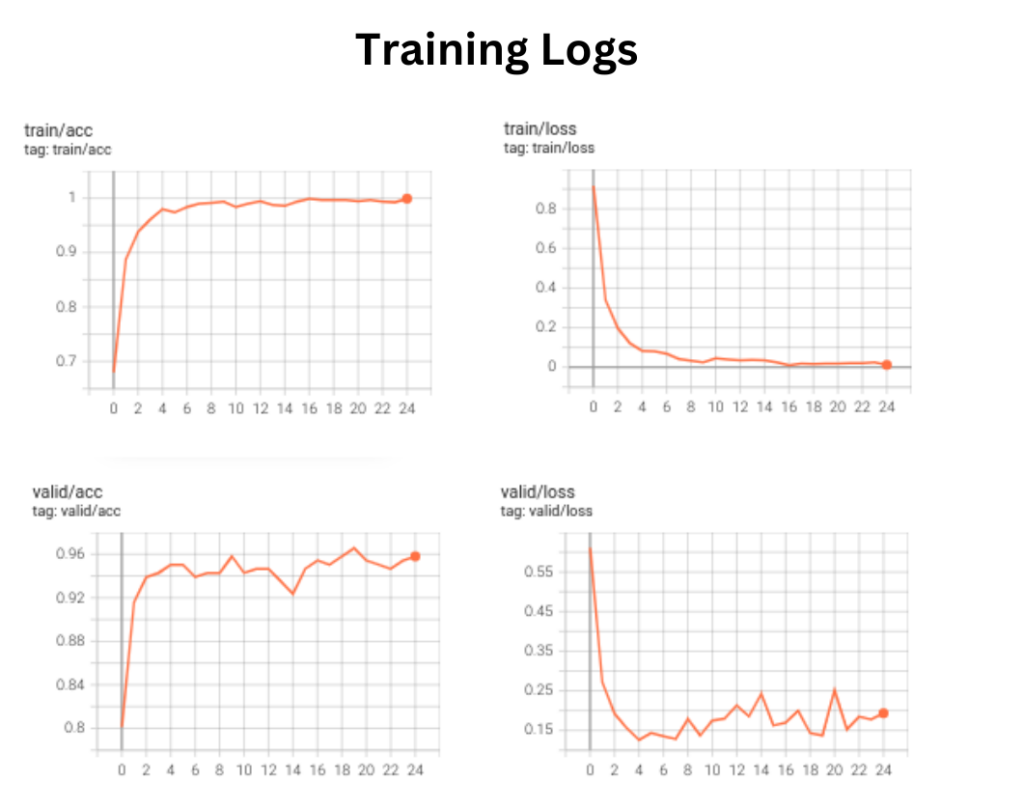
Note: The results are obtained after training on an RTX 3060 (6 GB) Laptop GPU.

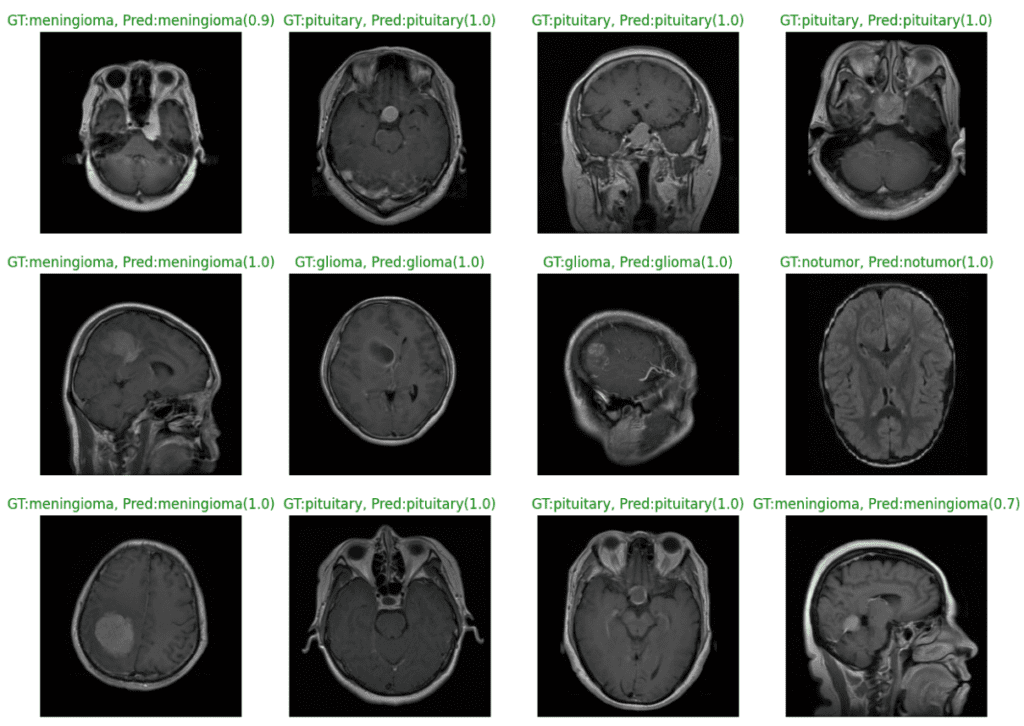
The plot below shows the model predictions from the fine-tuned EfficientNetv2 small model. We can see that the model classifies all the samples correctly with 100% confidence, barring a couple of instances.

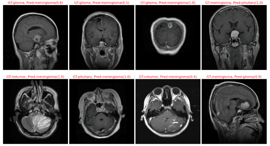
The following plot displays instances where our model has misclassified the image samples.

Class Activation Mapping (CAM)

So far in this article, we have performed image classification by fine-tuning a pre-trained imagenet classification model on a given dataset. We have seen how accurate the model is and also cases where it fails. However, we have not studied the results at a deeper level to understand what it is about a particular image that causes the model to make such predictions.

Much research on model interpretability has been carried out in the last decade, emphasizing visualizing the data within the model for making predictions. Class Activation Mapping (CAM) is one approach that gained traction and spurred several follow-on methods (GradCAM, GradCAM++, and HiResCAM). The output from such models tells us which portions of an input image are used for prediction. They show what the model focuses on (or “sees”) when making predictions for a particular class. It makes the decision-making of neural networks more transparent by providing us with a visual interpretation of the output.

In the following sections, we will first introduce the idea behind CAMs in the context of image classification. Then, we’ll cover the GradCAM model, which is a generalization of CAM.

CAM Architecture

The idea behind CAM is to take advantage of a specific type of convolutional neural network architecture that uses Global Average Pooling (GAP).  The architecture contains several convolutional layers for feature extraction, followed by a GAP layer and one fully connected layer that outputs classification scores. 

Classification Scores in CAM (or GradCAM)

Let’s first discuss how we compute the classification scores using this architecture. The last convolutional layer produces k feature maps in the diagram above. Just before the final output layer (softmax in the case of image classification), global average pooling is performed on the convolutional feature maps. Global average pooling turns a feature map into a single number by averaging the numbers in the feature map. After we perform Global Average Pooling, we have k numbers converted to classification scores using a single fully connected layer.

If we have k=3 feature maps, we’ll end up with k=3 numbers after global average pooling. We then use those numbers as features for a fully connected layer that produces the desired output (categorical or otherwise). For example, for a given class, we produce the class score, yc, as the weighted sum of the GAP numbers and the weights from the fully connected layer (for a given class) learned during training.

In the equation below, GAP(Ak) represents the global average pooling on the feature map Ak, a scalar.

Another way to look at this is that the GAP computation summarizes the information from each feature map, and then we learn the weights in the fully connected layer to make predictions. Therefore, the weighted sum of the feature maps for a given class should indicate which regions within the feature maps were most relevant to the prediction.

Note that the diagram only shows the connections in the fully connected layer for a single class to avoid clutter in the figure and simplify the indexing. In reality, the output from each node in the GAP layer is connected to each node in the output layer.

Class Activation Maps (CAM)

Now that we’ve covered the processing to produce the class scores, we’ll see that generating the class activation maps follows a similar computation. We compute the class activation heatmaps as the weighted sum of the activation maps.

This weighted sum is depicted in the graphic below after it was upsampled to match the size of the input image.

Note: One caveat regarding the architecture required for CAM is that it requires a GAP layer followed by a single fully connected layer to produce class activation maps.

In the next section below, we’ll cover GradCAM, a generalization of CAM that does not require a specific type of architecture.

Introduction to GradCAM

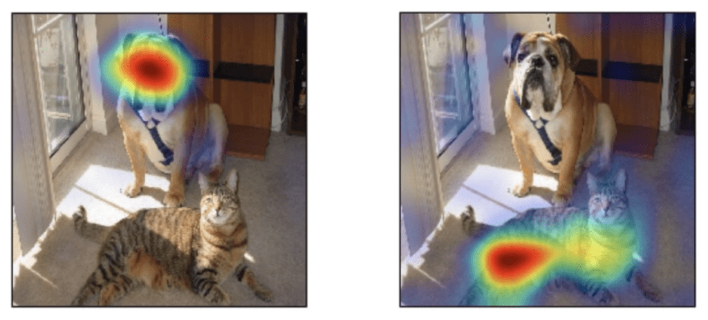
GradCAM, short for Gradient-weighted Class Activation Mapping, was introduced in the paper Grad-CAM: Gradient-weighted Class Activation Mapping by Selvaraju et al. GradCAM is more versatile than CAM because it can produce visual explanations of heatmaps for any arbitrary CNN architecture. The figures below from the research paper are examples of GradCAM output. 

GradCAM Architecture

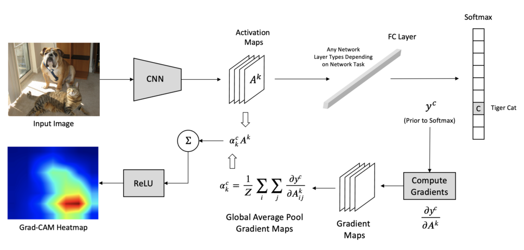
CAM and Grad-CAM differ in how the feature maps are weighted to compute the final heatmap.

In CAM, we weight these feature maps using the weights from the fully connected layer of the network. In Grad-CAM, feature maps are weighted using alpha values computed based on gradients. Therefore, Grad-CAM does not require a particular architecture since gradients can be computed through any kind of neural network layer we want. For example, the figure below depicts a single fully connected layer after the last convolutional layer. The following sections describe the processing pipeline depicted in the figure architecture diagram below.

Step 1: Gradient Computation in GradCAM

Each feature map from the last convolutional layer captures varying degrees of high-level information about the input image used to compute the final score for a given class. We aim to study the relationship between the feature maps and the output. For any given class, c , a change in the feature map would change the value of the score for that class. Therefore, the authors suggest that the gradient of the class score yc concerning the feature maps Ak should be used as the basis for computing an importance score to highlight regions in the input image that were used to make the prediction.

For the equation above, yc, is a scalar (predicted score before the softmax computation), and A^k is a two-dimensional feature map. So, the gradient is also a two-dimensional map with the exact spatial dimensions as the feature maps, A^k.

Step 2: Compute Alpha Values for GradCAM

In this step, we now perform global average pooling of the gradients over the width and height to obtain alpha values, which can be interpreted as importance values. The computation below produces k alpha values for each class, where Z is the total number of pixels in each feature map.

Step 3: Generate GradCAM Heatmap

The alpha values computed in the previous step are analogous to the weights in the final layer for the CAM approach, except that the alpha values were generated using gradients.

Similar to CAM, we can now compute a weighted sum of the activation maps where the weights are the alpha values computed above.

Finally, to compute the GradCAM heatmap, we pass the above-weighted sum through a ReLU (SiLU for EfficientNetv2) activation function to zero out any negative gradients.

The computation above will produce a coarse localization map that has the exact spatial dimensions as the feature maps, so to generate a final heatmap that can be overlayed on the image, the heatmap is simply upsampled to the same size as the input image and normalized to the range [0,1].

GradCAM Visualizations

Now that we have our fine-tuned model, we want to visualize a few samples of the validation data.

We begin by visualizing the GradCAM by calculating the gradients concerning the activations from the final Conv block (referenced by name: "features.7” as observed from the model summary). The following are the results.

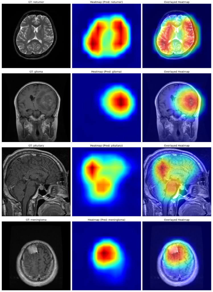
The dark red regions in the results correspond to highly activated regions within the image, while the blue ones correspond to regions with less activations. 

For the first image (the first raw), where there is no tumor, the heat maps are concentrated across both lobes of the brain, which is expected.

Let us now zoom in on the second image in the plot.

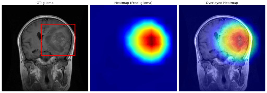
The region enclosed within the red box indicates the possible presence of a glioma. The same is clearly vindicated by the heat map obtained after GradCAM.

Before we move on to the third sample, let us quickly look at the fourth sample, where our fine-tuned model has focussed on the meningioma, as expected.

The third example is quite interesting.

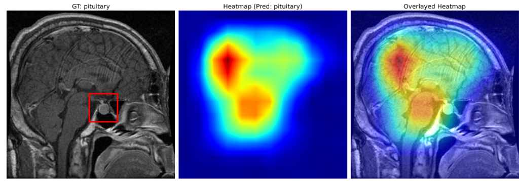
Instead of focusing entirely around the pituitary gland (enclosed in red), the heatmap is focused on the rear part of the cerebrum and partially around the spinal cord and the pituitary gland. However, the model has correctly classified the image as a pituitary tumor.

Let us see a few more visualizations.

Again, the emphasis from the heatmaps on the first two images is expected when the model correctly predicts the first image as a meningioma and no tumor in the second one.

However, for the third example, even though the model correctly classifies as pituitary, the focus region on the heatmaps after GradCAM is mainly around the cerebrum and partially around the cerebellum and the pituitary gland.

Looking at the above results, one might be biased towards thinking that images of the pituitary, even though the model can produce correct predictions, the heatmaps after GradCAM are only partially focussed on regions of pituitary glands. 

Well, that may be the case for pituitary tumors; however, the same can be extended for other class examples as well. For instance, take a look at the example of glioma below.

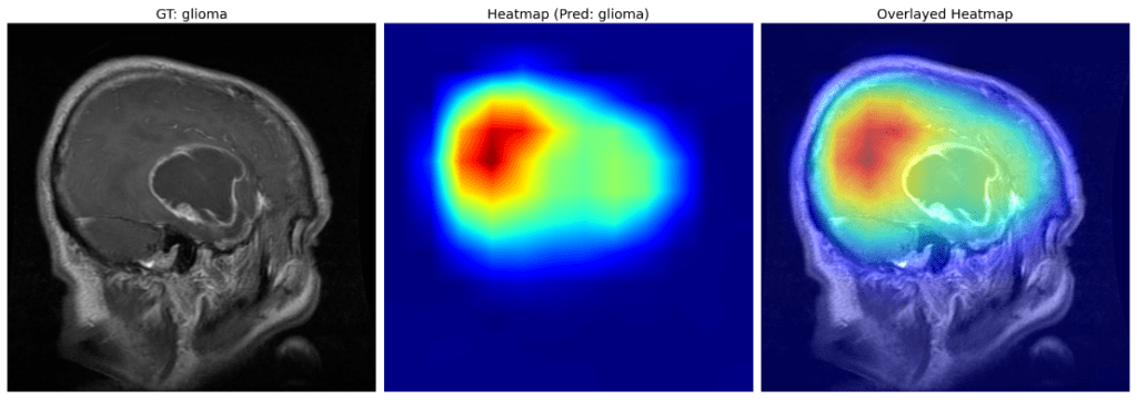
The heatmaps above indicate the focus region is mainly around the “bulge” of the brain (probably caused by the glioma) rather than the glioma itself.

The instances from the heatmaps discussed above might be attributed to the gradient averaging step used by GradCAM. More recent work, such as HighResCAM, produces more relevant results. HiResCAM addresses this problem using an element-wise product between the raw gradients and the feature maps. HiResCAM accomplishes all the same purposes as GradCAM, with the benefit that HiResCAM is probably guaranteed to highlight only the regions where the model is used to make each prediction.

For example, the GradCAM heatmaps are computed for an intermediate convolution layer from the EfficienNet model. Specifically, we use the "features.6.5” layer from the EfficientNetv2 small model.

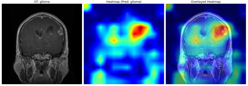
As you can see in the image instance above, the information from earlier convolutional layers in the network seems to contain information related to lower-level patterns rather than higher-level contextual information. The heatmaps produced seem to be more closely tied to objects of each class.

Did you find the results insightful? If so, you can scroll through the detailed discussion of the complete training and GradCAM pipeline in the article.

Summary and Conclusion

To summarize this article, we started by fine-tuning EfficientNetv2 small, a popular ImageNet pre-trained classification model. The dataset used for our experiments was the Brain MRI Scans data comprising four categories of instances, viz-a-viz: glioma, meningioma, no-tumor, and pituitary, where we achieved a pretty descent accuracy of around 96.6% in the validation data.

Next, we introduced the general topic of model interpretability and references to several approaches developed over the past several years to provide visual explanations for why CNNs make the predictions they do. We covered the basic idea behind Class Activation Mapping and showed how GradCAM is a generalization of CAM that uses gradients to produce the final result. We then deduced the results from the heatmaps generated after computing the GradCAM from our fine-tuned model.

We also discussed a few cases where GradCAM is known to highlight regions of an image that were not used for prediction. This finding gave rise to another approach called HiResCAM, which uses a slightly different approach for computing the gradients and might mitigate the problem with GradCAMs. 

We’d love to hear from you! Share your insights and reactions in the comments below. Your thoughts are valuable to us, and we’re excited to engage in a lively discussion with you!

References

• Brain MRI Scans Dataset for Brain Tumor Classification
• Grad-CAM: Visual Explanations from Deep Networks via Gradient-based Localization
• Use HiResCAM instead of Grad-CAM for faithful explanations of convolutional neural networks