As AI engineers, we’re always building cool machine learning and deep learning models, right? But then we hit the big question: “Where do we deploy these models so that end-users can actually use them?” In this article, we’ll explore whether integrating Gradio with OpenCV DNN might be the solution we’re looking for. Could this be the perfect solution for creating lightweight, efficient web applications with real-time inference capabilities? Let’s explore this intriguing possibility and see if it can truly be the game-changer we hope for.
To see the web app we made, scroll down to the inference part of the article or click here to see them immediately.
All the code discussed in this article is free to grab. Just hit the Download Code button to get started.
What is the OpenCV DNN Module?
OpenCV, the world’s largest computer vision library, offers a powerful tool for deep learning model inference, the OpenCV DNN Module[1]. This module boasts extensive model support across popular frameworks like Tensorflow, Pytorch, ONNX, Caffe, and more. What’s even better is its highly optimized for Intel processors, allowing for decent FPS even with just your CPU. This means you can run inference of deep learning models without the need for costly GPUs or extensive hardware optimization.
You can explore more about OpenCV DNN in our detailed blog post.
Introduction to Gradio
Gradio[2] is a Python package that allows us to build a Graphical User Interface(GUI) for our machine-learning projects. It’s developed and maintained by HuggingFace. As AI Engineers, we are more involved in Deep Learning and Computer Vision, and building any web application out of our ML model becomes a hectic task.
Gradio provides us with custom UI components that are out of the box to build and enhance our web applications, using just a few lines of Python and without extensive knowledge of HTML, CSS, or JavaScript.
You can build any ML demo using Gradio and Host it in HuggingFace Spaces to showcase your creativity. You can learn more about gradio by reading our article about Deploying a Deep Learning Model using Hugging Face Spaces and Gradio.
Gradio with OpenCV DNN – Overview
In this article, we will focus on creating interfaces for two renowned object detection models: MobileNet SSD and YOLOv3. Here’s how we’ll structure the web application:
- Tabbed Interface Setup:
- We will create a single tabbed interface that houses both image and video inference functionalities.
- Image Inference Interface:
- This part of the interface will have two tabs: one for input and another for output.
- A checkbox will be provided to allow the user to choose between MobileNet SSD and YOLOv3 models for image detection.
- Video Inference Interface:
- This section will be divided into three tabs:
- The first tab will be for video input, where users can upload or select a video.
- The second tab will display live inference, showing real-time object detection on the uploaded video.
- The third tab will be for the output, presenting the final annotated video after processing.
- This section will be divided into three tabs:
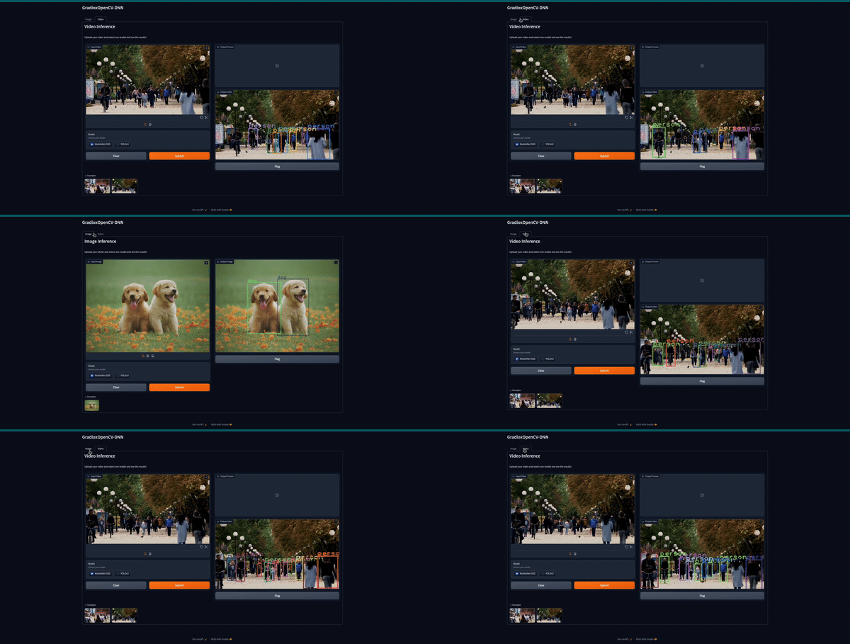
The best part is that we can make this complicated UI using Gradio, OpenCV DNN, and Python.
Gradio with OpenCV DNN – MoblieNet SSD
MobileNet SSD is one of the popular object detection models developed for fast and lightweight inference on edge devices, such as mobile phones or less powerful CPUs.

MobileNet[3] is a deep neural network architecture designed for faster image classification inference on resource-constrained devices. Its core innovation is the use of depth-wise separable convolutions, which significantly reduce the number of parameters and computational costs compared to traditional convolutional layers. It should be noted that the first layer in MobileNet is a standard convolutional layer, not a depth-wise separable convolution, which is used to reduce the dimensionality and initially capture basic features.
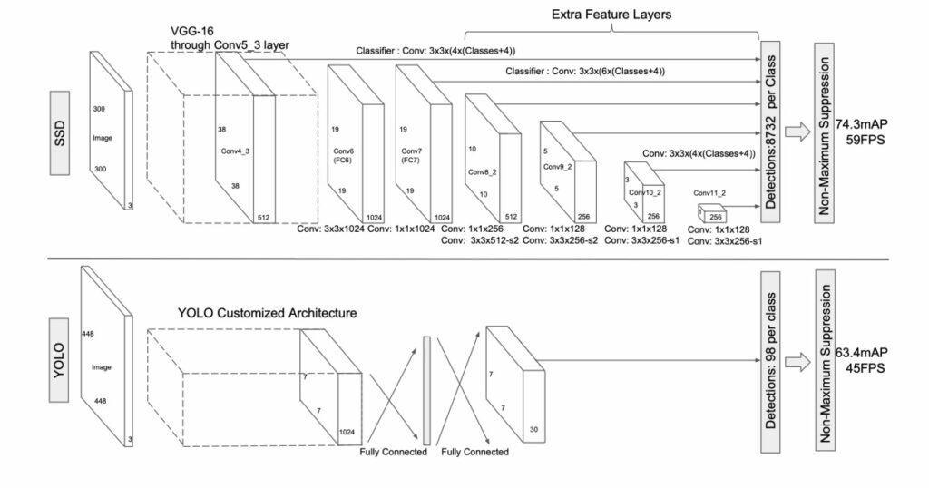
The Google Research team introduced the 2nd part of the model Single Shot MultiBox Detector (SSD)[4], which detects objects in an image in a single forward pass (unlike RCNN family detectors). The SSD approach is based on a feed-forward convolutional network that predicts a collection of bounding boxes and scores for the detected objects. SSD is designed to be independent of the base network and run on top of any backbone, such as VGG, YOLO, or MobileNet.
MobileNet-SSD combines the MobileNet as the backbone and SSD as the head to make real-time object detection even faster and lightweight.
Gradio with OpenCV DNN – YOLOv3
YOLOv3[5] is the third version in the YOLO series, renowned for its effectiveness in object detection tasks. This model leverages DarkNet-53 as its core for extracting features, which is a deep convolutional neural network composed of 53 layers. Its architectural design features alternating (1×1) and (3×3) convolutional layers, integrated with skip or residual connections, drawing inspiration from the ResNet architecture. This structure aids in mitigating the vanishing gradient problem, thereby enhancing the learning capability for deep networks.
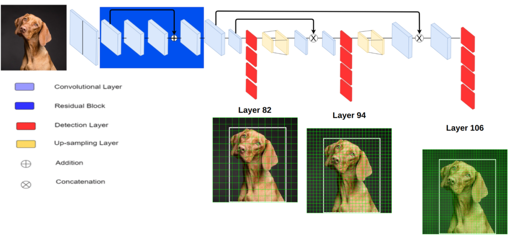
YOLOv3 stands out for its ability to make predictions at three distinct scales or resolutions, which enhances its detection accuracy across various object sizes. Unlike previous versions that used a single softmax layer for class prediction, YOLOv3 employs multiple independent logistic classifiers for each class. This approach allows for the detection of multiple objects within the same grid cell, improving the model’s performance in detecting a wide range of objects simultaneously.
Now that we are done covering the basics of the models we’ll be using, let’s focus on coding and getting our object detection app running in Gradio.
Gradio with OpenCV DNN – Code Pipeline
Our code pipeline consists of 3 Python scripts:
mbnet.py– Script to get and process detections of MobileNet SSD using OpenCV DNNyolov3.py– Script to get and process detection of YOLOv3 using OpenCV DNNapp.py– Combine both scripts in a single web app using Gradio
Gradio with OpenCV DNN – mbnet.py
We will load the MobileNet-SSD model using the OpenCV DNN Module in the below script. We have also included the code for processing the detections made by the model.
import cv2
import numpy as np

def load_model():
    # Load the trained model from files
    model = cv2.dnn.readNet(model='frozen_inference_graph.pb',
                            config='ssd_mobilenet_v2_coco_2018_03_29.pbtxt.txt',
                            framework='TensorFlow')
    # Load class names from file
    with open('object_detection_classes_coco.txt', 'r') as f:
        class_names = f.read().split('\n')
    # Generate random colors for the bounding boxes
    COLORS = np.random.uniform(0, 255, size=(len(class_names), 3))
    return model, class_names, COLORS

def load_img(img_path):
    # Load and resize the image
    img = cv2.imread(img_path)
    img = cv2.resize(img, None, fx=0.4, fy=0.4)
    height, width, channels = img.shape
    return img, height, width, channels

def detect_objects(img, net):
    # Prepare the image for the model
    blob = cv2.dnn.blobFromImage(img, size=(300, 300), mean=(104, 117, 123), swapRB=True)
    net.setInput(blob)
    outputs = net.forward()
    return blob, outputs

def get_box_dimensions(outputs, height, width):
    boxes = []
    class_ids = []
    # Loop through the detections and store the box coordinates and class IDs
    for detect in outputs[0,0,:,:]:
        scores = detect[2]
        class_id = detect[1]
        if scores > 0.3:  # Filter out weak detections
            center_x = int(detect[0] * width)
            center_y = int(detect[1] * height)
            w = int(detect[5] * width)
            h = int(detect[6] * height)
            x = int((detect[3] * width))
            y = int((detect[4] * height))
            boxes.append([x, y, w, h])
            class_ids.append(class_id)
    return boxes, class_ids

def draw_labels(boxes, colors, class_ids, classes, img):
    font = cv2.FONT_HERSHEY_PLAIN
    # Draw bounding boxes and labels on the image
    for i in range(len(boxes)):
        x, y, w, h = boxes[i]
        label = classes[int(class_ids[0])-1]
        color = colors[i]
        cv2.rectangle(img, (x,y), (w,h), color, 5)
        cv2.putText(img, label, (x, y - 5), font, 5, color, 5)
    return img

def image_detect(img_path):
    # Load the model, classes, and colors
    model, classes, colors = load_model()
    # Load, detect and draw bounding boxes on the image
    image, height, width, channels = load_img(img_path)
    blob, outputs = detect_objects(image, model)
    boxes, class_ids = get_box_dimensions(outputs, height, width)
    image1 = draw_labels(boxes, colors, class_ids, classes, image)
    return image1

# Cleanup and release resources
cv2.destroyAllWindows()
After the library imports, we use cv2.dnn.readNet() to load the MobileNet SSD model. We are using the TensorFlow model, which requires the model weights file frozen_inference_graph.pb and a protobuf text file ssd_mobilenet_v2_coco_2018_03_29.pbtxt.txt containing the model configuration.
Then, we defined different functions for different tasks:
load_model - to load the model
load_img - load the image file
detect_objects - get detection using the model
get_box_dimensions - process the detection
draw_labels - annotate the detections in input frame
In detect_objects, we defined the blob, set input for the blob, and ran the forward pass.
And the output shape we got:
output-shape = (1, 1, 100, 7)

[[[[ 0.00000000e+00  1.80000000e+01  9.99486804e-01  5.01647472e-01

    2.09531128e-01  7.55192161e-01  8.21747720e-01]]]]
Let’s understand the detection output of the model one by one:
- The first dimension 1 in the shape (1, 1, 100, 7): It’s part of the output dimensions that OpenCV’s DNN module uses for its outputs.
- The second dimension 1: It is often a placeholder or could be part of the network’s output dimension.
- The third dimension 100: It represents the number of detections made by the network. SSD models often have a fixed number of potential detections per image, including both true and false positives and many low-confidence detections.
- The fourth dimension 7: It represents the normalized data for each detection, typically including the batch index (indicating which image in the batch the detection belongs to), class ID, confidence score, and bounding box coordinates (x, y, width, height).
def get_box_dimensions(outputs, height, width):
    boxes = []
    class_ids = []
    # Loop through the detections and store the box coordinates and class IDs
    for detect in outputs[0,0,:,:]:
        scores = detect[2]
        class_id = detect[1]
        if scores > 0.3:  # Filter out weak detections
            center_x = int(detect[0] * width)
            center_y = int(detect[1] * height)
            w = int(detect[5] * width)
            h = int(detect[6] * height)
            x = int((detect[3] * width))
            y = int((detect[4] * height))
            boxes.append([x, y, w, h])
            class_ids.append(class_id)
    return boxes, class_ids
We use the get_box_dimensions function to extract specific data from the output tensor:
- First, we use array slicing and indexing techniques to extract Class ID, Confidence score, and Coordinate values from the tensor.
- Next, convert the normalized output coordinates into pixel values by multiplying them with the input frame’s height and width.
- Finally, return the identified classes along with their corresponding bounding boxes from the function.
- After that, we use the draw_labels function to annotate the input frames with the bounding box values and add the class name using
cv2.putText.
Gradio with OpenCV DNN – yolov3.py
We will load the YOLOv3 model trained on the Darknet architecture and process the outputs in this script.
import cv2
import numpy as np

# Load YOLO model from disk
def load_yolo():
    net = cv2.dnn.readNet("yolov3.weights", "yolov3.cfg")
    classes = []
    with open("coco.names", "r") as f:
        classes = [line.strip() for line in f.readlines()]

    # Get the output layer names used for the forward pass
    output_layers = [layer_name for layer_name in net.getUnconnectedOutLayersNames()]
    # Generate random colors for each class
    colors = np.random.uniform(0, 255, size=(len(classes), 3))
    return net, classes, colors, output_layers

# Load an image from disk and resize
def load_image(img_path):
    img = cv2.imread(img_path)
    img = cv2.resize(img, None, fx=0.4, fy=0.4)
    height, width, channels = img.shape
    return img, height, width, channels

# Start the webcam
def start_webcam():
    cap = cv2.VideoCapture(0)
    return cap

# Display the blob for debugging
def display_blob(blob):
    for b in blob:
        for n, imgb in enumerate(b):
            cv2.imshow(str(n), imgb)

# Detect objects using YOLO
def detect_objects_yolo(img, net, outputLayers):
    blob = cv2.dnn.blobFromImage(img, scalefactor=0.00392, size=(320, 320), mean=(0, 0, 0), swapRB=True, crop=False)
    net.setInput(blob)
    outputs = net.forward(outputLayers)
    for i, out in enumerate(outputs):
        print(i, np.array(out).shape)
    return blob, outputs

#  Process the network's output to extract bounding boxes, confidences, and class IDs.
def get_box_dimensions_yolo(outputs, height, width):

    boxes = []
    confs = []
    class_ids = []
    # Iterate through each detection
    for output in outputs:
        for detect in output:
            scores = detect[5:]  # Exclude first 4 bounding box parameters
            class_id = np.argmax(scores)  # Find the class with the highest score
            conf = scores[class_id]  # Confidence of the class
            if conf > 0.3:  # Filter out weak detections
                center_x = int(detect[0] * width)
                center_y = int(detect[1] * height)
                w = int(detect[2] * width)
                h = int(detect[3] * height)
                x = int(center_x - w / 2)
                y = int(center_y - h / 2)
                boxes.append([x, y, w, h])
                confs.append(float(conf))
                class_ids.append(class_id)
    return boxes, confs, class_ids

# Draw bounding boxes and labels on the image
def draw_labels_yolo(boxes, confs, colors, class_ids, classes, img):
    indexes = cv2.dnn.NMSBoxes(boxes, confs, 0.5, 0.4)
    font = cv2.FONT_HERSHEY_PLAIN
    for i in range(len(boxes)):
        if i in indexes:
            x, y, w, h = boxes[i]
            label = str(classes[class_ids[i]])
            color = colors[i]
            cv2.rectangle(img, (x, y), (x + w, y + h), color, 5)
            cv2.putText(img, label, (x, y - 5), font, 5, color, 5)
    return img

# Process an image to detect and label objects
def image_detect_yolo(img_path):
    model, classes, colors, output_layers = load_yolo()
    image, height, width, channels = load_image(img_path)
    blob, outputs = detect_objects_yolo(image, model, output_layers)
    boxes, confs, class_ids = get_box_dimensions_yolo(outputs, height, width)
    image = draw_labels_yolo(boxes, confs, colors, class_ids, classes, image)
    return image

# Clean up any open windows
cv2.destroyAllWindows()
Similar to mbnet.py, we import the libraries and use cv2.dnn.readNet to load the YOLOv3 model. We use the Darknet pre-trained model, which requires the model weights file yolov3.weights and a config file yolov3.cfg containing the model configuration.
Then, we defined different functions for different tasks:
load_yolo - to load the model
load_img - load the image file
detect_objects_yolo - get detection using the model
get_box_dimensions_yolo - process the detection
draw_labels_yolo - annotate the detections in input frame
In detect_objects_yolo, we defined the blob, set input for the blob, and ran the forward pass.
And the output shape we got:
Output-shape:

0 (300, 85)
1 (1200, 85)
2 (4800, 85)

array([[0.05896439, 0.03014819, 0.3622023 , ..., 0.        , 0.        ,
       0.        ],
      [0.06667177, 0.0431477 , 0.29185498, ..., 0.        , 0.        ,
       0.        ],
      [0.06918813, 0.03046303, 1.3190577 , ..., 0.        , 0.        ,
       0.        ],
      ...,
      [0.9403159 , 0.9377915 , 0.61475384, ..., 0.        , 0.        ,
       0.        ],
      [0.9511486 , 0.9536129 , 0.43074816, ..., 0.        , 0.        ,
       0.        ],
      [0.96671116, 0.9561311 , 1.0985503 , ..., 0.        , 0.        ,
       0.        ]], dtype=float32)
Yolov3 gives output in 3 different output layers as (N,85) where:
- N – the total number of boxes predicted by each layer
- 85:
- 4 numbers for the bounding box (center x, center y, width, height),
- 1 number for the objectness score (confidence that an object is present),
- 80 numbers for the class probabilities (the COCO dataset with 80 classes).
So, if we break down all the output layers:
- 0 (300, 85): The first scale (often the largest objects in terms of relative size to the image) with 300 predictions, each containing 85 pieces of information.
- 1 (1200, 85): The second scale (medium objects) with 1200 predictions, each with 85 pieces of information.
- 2 (4800, 85): The third scale (smallest objects) with 4800 predictions, each with 85 pieces of information.
def get_box_dimensions_yolo(outputs, height, width):
    """
    Process the network's output to extract bounding boxes, confidences, and class IDs.
    Returns lists of boxes, confidences, and class IDs.
    """
    boxes = []
    confs = []
    class_ids = []
    # Iterate through each detection
    for output in outputs:
        for detect in output:
            scores = detect[5:]  # Exclude first 4 bounding box parameters
            class_id = np.argmax(scores)  # Find the class with the highest score
            conf = scores[class_id]  # Confidence of the class
            if conf > 0.3:  # Filter out weak detections
                center_x = int(detect[0] * width)
                center_y = int(detect[1] * height)
                w = int(detect[2] * width)
                h = int(detect[3] * height)
                x = int(center_x - w / 2)
                y = int(center_y - h / 2)
                boxes.append([x, y, w, h])
                confs.append(float(conf))
                class_ids.append(class_id)
    return boxes, confs, class_ids
Then, we use the get_box_dimensions_yolo() function to extract the class ID, confidence score, and coordinate values from the output tensor. We simply use array slicing and indexing to extract those values, multiplying the input frame height and width with the normalized output coordinates into pixel values. Then, we return these bounding boxes, prediction confidences, and the respective class IDs.
After that, we use the draw_labels function() to annotate the input frames with the bounding box values and add the class name using cv2.putText.
Gradio with OpenCV DNN – app.py
In the app.py script, we will import all the functions we defined in mbnet.py and yolov3.py and create the gradio web app using all the functions.
import cv2
import numpy as np
import gradio as gr
from mbnet import load_model, detect_objects, get_box_dimensions, draw_labels, load_img
from yolov3 import load_image, load_yolo, detect_objects_yolo, get_box_dimensions_yolo, draw_labels_yolo
After importing all the libraries, we will create two functions for the image and video inference code pipeline:
Img_inf
# Image Inference Function
def img_inf(img, model):
    # Choose the model based on user selection
    if model == "MobileNet-SSD":
        model, classes, colors = load_model()  # Load the MobileNet-SSD model
        image, height, width, channels = load_img(img)  # Load and preprocess the image
        blob, outputs = detect_objects(image, model)  # Detect objects in the image
        boxes, class_ids = get_box_dimensions(outputs, height, width)  # Get the bounding boxes
        image1 = draw_labels(boxes, colors, class_ids, classes, image)  # Draw labels on the image
        return cv2.cvtColor(image1, cv2.COLOR_BGR2RGB)  # Return the processed image in RGB format
    else:
        model, classes, colors, output_layers = load_yolo()  # Load the YOLO model
        image, height, width, channels = load_image(img)  # Load and preprocess the image
        blob, outputs = detect_objects_yolo(image, model, output_layers)  # Detect objects with YOLO
        boxes, confs, class_ids = get_box_dimensions_yolo(outputs, height, width)  # Get bounding boxes
        image = draw_labels_yolo(boxes, confs, colors, class_ids, classes, image)  # Draw labels on the image
        return cv2.cvtColor(image, cv2.COLOR_BGR2RGB)  # Return the processed image in RGB format
The img_inf function will take the input image and the model name and will return the output image. First, we create an if-else statement for the model name, and we will call the specific functions according to the model. Then, we set the code pipeline or algorithm in a step-by-step manner:
- First, we will load the model using
load_modelorload_yolo
- Then, we will load the input image using
load_img
- Then, with the input image and model, we will extract the model outputs using
detect_objectsordetect_objects_yolo
- After that, with the outputs, we will extract the bounding box coordinates and class IDs using
get_box_dimensionsordetect_objects_yolo
- Finally, we will annotate the input image with the bounding boxes and class name using bounding box coordinates and class IDs with
draw_labelsordraw_labels_yolo
We will return the final output image at the end.
# Setup for Gradio interface
model_name = gr.Radio(["MobileNet-SSD", "YOLOv3"], value="YOLOv3", label="Model", info="choose your model")
inputs_image = gr.Image(type="filepath", label="Input Image")
outputs_image = gr.Image(type="numpy", label="Output Image")

# Create Gradio Interface for Image Inference
interface_image = gr.Interface(
    fn=img_inf,
    inputs=[inputs_image, model_name],
    outputs=outputs_image,
    title="Image Inference",
    description="Upload your photo and select one model and see the results!",
    examples=[["sample/dog.jpg"]],
    cache_examples=False,
)
Now, we will create the image inference tab using gradio. We will create a button-select component with gr.Radio and for input and output image, we will create two placeholders with gr.Image component. Then, we will create the final interface using gr.Interface and pass the img_inf function.
vid_inf
# Video Inference Function
def vid_inf(vid, model_type):
    # Choose the model based on user selection
    if model_type == "MobileNet-SSD":
        cap = cv2.VideoCapture(vid)  # Start capturing video from the file
        frame_width = int(cap.get(3))  # Get video width
        frame_height = int(cap.get(4))  # Get video height
        fps = int(cap.get(cv2.CAP_PROP_FPS))  # Get frames per second
        frame_size = (frame_width, frame_height)  # Determine the size of video frames
        fourcc = cv2.VideoWriter_fourcc(*"mp4v")  # Define codec
        output_video = "output_recorded.mp4"  # Output file name

        out = cv2.VideoWriter(output_video, fourcc, fps, frame_size)  # Create VideoWriter object

        model, classes, colors = load_model()  # Load the MobileNet-SSD model
        while cap.isOpened():
            ret, frame = cap.read()
            if ret:
                height, width, channels = frame.shape  # Get frame dimensions
                blob, outputs = detect_objects(frame, model)  # Detect objects in the frame
                boxes, class_ids = get_box_dimensions(outputs, height, width)  # Get bounding boxes
                frame = draw_labels(boxes, colors, class_ids, classes, frame)  # Draw labels on the frame
                out.write(frame)  # Write the frame to the output video file
                yield cv2.cvtColor(frame, cv2.COLOR_BGR2RGB), None  # Yield the processed frame
            else:
                break

        cap.release()  # Release the video capture object
        out.release()  # Release the video writer object
        cv2.destroyAllWindows()  # Close all OpenCV windows
        yield None, output_video  # Return the output video file

    else:
        # Similar processing for YOLO model as above, with YOLO-specific functions
        cap = cv2.VideoCapture(vid)
        frame_width = int(cap.get(3))
        frame_height = int(cap.get(4))
        fps = int(cap.get(cv2.CAP_PROP_FPS))
        frame_size = (frame_width, frame_height)
        fourcc = cv2.VideoWriter_fourcc(*"mp4v")
        output_video = "output_recorded.mp4"

        out = cv2.VideoWriter(output_video, fourcc, fps, frame_size)

        model, classes, colors, output_layers = load_yolo()
        while cap.isOpened():
            ret, frame_y = cap.read()
            if ret:
                height, width, channels = frame_y.shape
                blob, outputs = detect_objects_yolo(frame_y, model, output_layers)
                boxes, confs, class_ids = get_box_dimensions_yolo(outputs, height, width)
                frame_y = draw_labels_yolo(boxes, confs, colors, class_ids, classes, frame_y)
                out.write(frame_y)
                yield cv2.cvtColor(frame_y, cv2.COLOR_BGR2RGB), None
            else:
                break

        cap.release()
        out.release()
        cv2.destroyAllWindows()
        yield None, output_video
The vid_inf function will take the input video and the model name and will return the output video frames and final output video. First, we create an if-else statement for the model name, and we will call the specific functions according to the model. Then, we set the code pipeline or algorithm in a step-by-step manner:
- First, we will create the
VideoCaptureandVideoWriterobject
- Then, we will load the model using
load_modelorload_yolo
- After that, we read all the video frames using
cap.readand will pass those into the pipeline.
- Then, with the video frames and model, we will extract the model outputs using
detect_objectsordetect_objects_yolo - After that, with the outputs, we will extract the bounding box coordinates and class IDs using
get_box_dimensionsordetect_objects_yolo
- Finally, we will annotate the input image with the bounding boxes and class name using bounding box coordinates and class IDs with
draw_labelsordraw_labels_yolo
We will return the output frames and the final output video.
# Setup for Gradio interface
model_name = gr.Radio(["MobileNet-SSD", "YOLOv3"], value="YOLOv3", label="Model", info="choose your model")
input_video = gr.Video(sources=None, label="Input Video")
output_frame = gr.Image(type="numpy", label="Output Frames")
output_video_file = gr.Video(label="Output video")

# Create Gradio Interface for Video Inference
interface_video = gr.Interface(
    fn=vid_inf,
    inputs=[input_video, model_name],
    outputs=[output_frame, output_video_file],
    title="Video Inference",
    description="Upload your video and select one model and see the results!",
    examples=[["sample/video_1.mp4"], ["sample/person.mp4"]],
    cache_examples=False,
)
Now, we will create the video inference tab using gradio. We will create a button to select components with gr.Radio , and for input and output video, we will create two placeholders with gr.Video components. But we want to show the live output frame inference so that we will add another gr.Image component. Then, we will create the final interface using gr.Interface and pass the video_inf function.
# Combine both interfaces in a tabbed layout
gr.TabbedInterface(
    [interface_image, interface_video], tab_names=["Image", "Video"], title="GradioxOpenCV-DNN"
).queue().launch()
Finally, we will create a tabbed interface for image and video inference with gr.TabbedInterface and pass both the image and video inference tabs.
We are done with building our web app.
Inference with Gradio
Now, we will run our Gradio web app and check out its functionalities. First, we’ll run inference on an image in the Image inference tab:
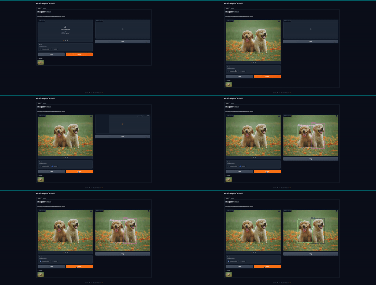
The interface features a section on the left for uploading an input image and selecting the model through a dropdown button. Upon clicking the submit button, the model processes the input, and the resulting output image is displayed on the right side of the interface.
Next up is Video Inference:
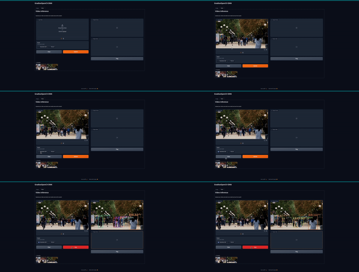
On the left side of our interface, similar to the image inference tab, we have two distinct sections: one for uploading the input video and another for selecting the model via a button. On the right side, we have two output sections. The first section is dedicated to displaying live inference results through the output video frames.
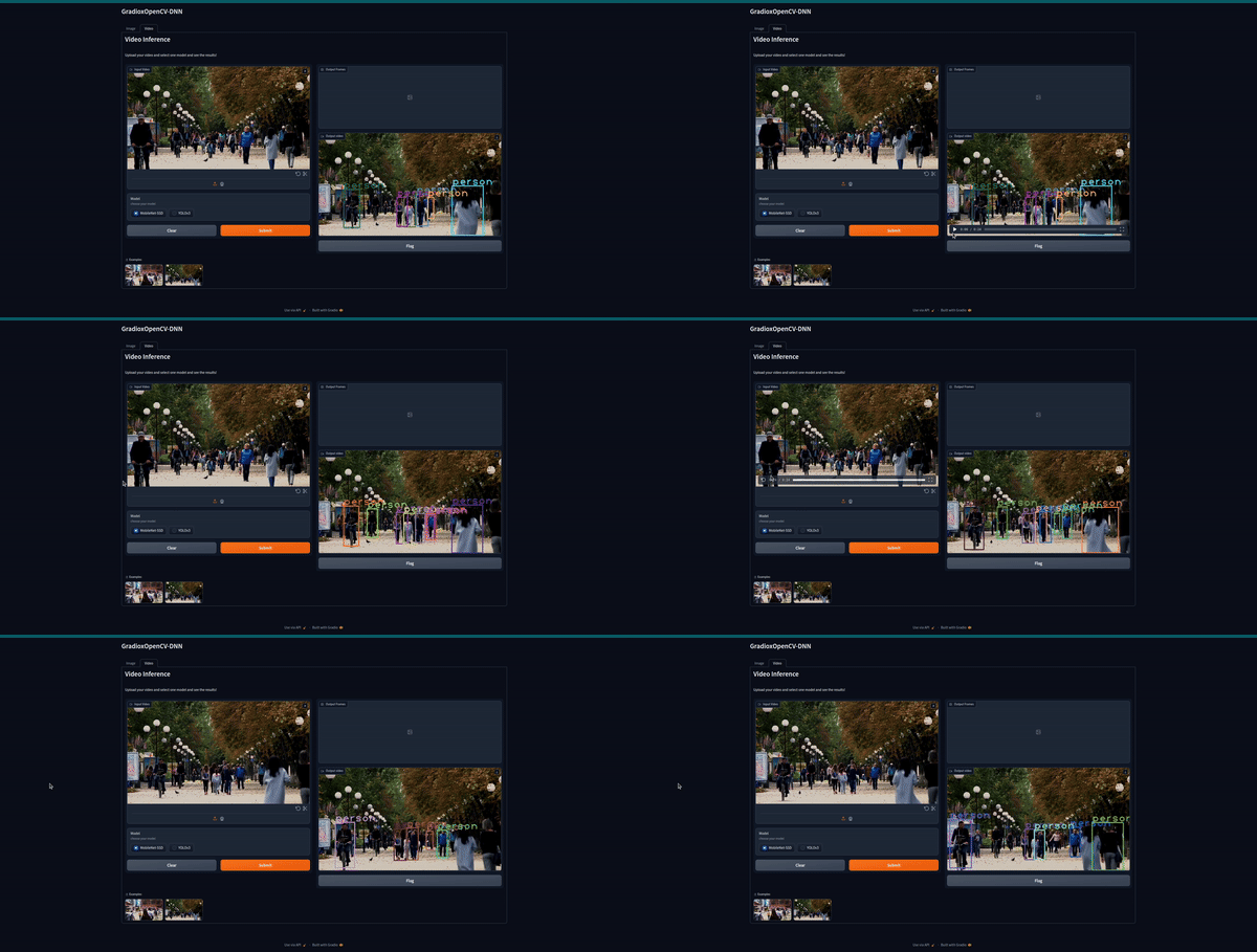
Next, there is a section dedicated to showing the final processed output video, presenting the completed analysis.
Concludingly, we designed a tabbed interface that consolidates both image and video processing capabilities in one unified location.

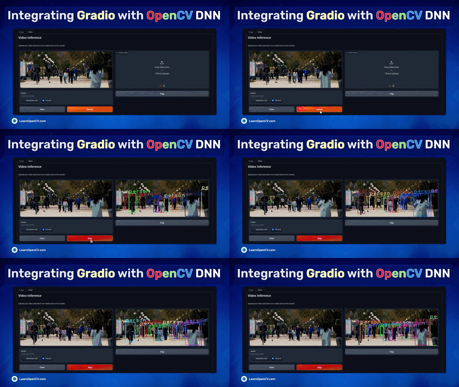
We developed this cool web app using Gradio with OpenCV DNN. The app has been deployed on Hugging Face Spaces, and we invite you to try it out by clicking the button below:
Now, let’s have a quick walk-through of the main components of this implementation.
Key takeaways
- Introduction to OpenCV DNN: The OpenCV DNN module is a powerful tool for deep learning model inference. It supports a variety of frameworks and is optimized for performance, even on less powerful hardware. This module lets developers quickly execute complex deep learning models, highlighting their importance in the computer vision ecosystem.
- Introduction to Gradio: Gradio is a Python library that simplifies the creation of graphical user interfaces for machine learning models. It allows developers to quickly build and share interactive demos of their models, facilitating easier experimentation, testing, and showcasing of AI models’ capabilities without deep knowledge of web technologies.
- Integration of Gradio with OpenCV DNN: Combining Gradio with OpenCV DNN module enables developers to build interactive web applications for object detection models. This integration provides a straightforward approach to visualize and interact with the model’s predictions, enhancing the accessibility and user experience of AI-powered applications.
- Real-time Inference on Images and Videos: The integrated system of Gradio with OpenCV DNN allows for real-time inference on images and videos, demonstrating the practical application of these technologies in dynamic environments. This capability is crucial for developing applications that require immediate processing and analysis, such as in surveillance, automotive, and various forms of live media analysis.
Conclusion
In conclusion, integrating Gradio with OpenCV DNN makes creating fast, easy-to-use web apps for real-time analysis straightforward. This blend offers a simple way to apply advanced AI, allowing for quick, interactive experiences. With Gradio and OpenCV DNN, developers can efficiently bring powerful vision technology to users everywhere, simplifying advanced AI use.


100K+ Learners
Join Free OpenCV Bootcamp3 Hours of Learning