


In this post, we will learn how to perform feature-based image alignment using OpenCV. We will share code in both C++ and Python.
We will demonstrate the steps by way of an example in which we will align a photo of a form taken using a mobile phone to a template of the form. The technique we will use is often called “feature based” image alignment because in this technique a sparse set of features are detected in one image and matched with the features in the other image. A transformation is then calculated based on these matched features that warps one image on to the other.
Previously, we had covered area based image alignment in ECC Image Alignment. If you have not read that post, I recommend you do it because it covers a very cool application involving the history of photography.
What is Image Alignment or Image Registration?
In many applications, we have two images of the same scene or the same document, but they are not aligned. In other words, if you pick a feature (say a corner) on one image, the coordinates of the same corner in the other image is very different.
Image alignment (also known as image registration) is the technique of warping one image ( or sometimes both images ) so that the features in the two images line up perfectly.
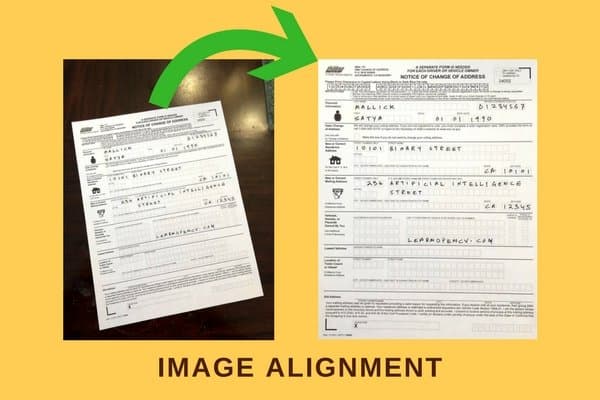
In the above example, we have a form from the Department of Motor Vehicles on the left. The form was printed, filled out and then photographed using a mobile phone (center). In this document analysis application, it makes sense to first align the mobile photo of the form with the original template before doing any analysis. The output after alignment is shown on the right image.


Applications of Image Alignment
Image alignment has numerous applications.
In many document processing applications, the first step is to align the scanned or photographed document to a template. For example, if you want to write an automatic form reader, it is a good idea to first align the form to its template and then read the fields based on a fixed location in the template.
In some medical applications, multiple scans of a tissue may be taken at slightly different times and the two images are registered using a combination of techniques described in this tutorial and the previous one.
The most interesting application of image alignment is perhaps creating panoramas. In this case the two images are not that of a plane but that of a 3D scene. In general, 3D alignment requires depth information. However, when the two images are taken by rotating the camera about its optical axis (as in the case of panoramas), we can use the technique described in this tutorial to align two images of a panorama.
Image Alignment : Basic Theory
At the heart of image alignment techniques is a simple 3×3 matrix called Homography. The Wikipedia entry for homography can look very scary.
Worry you should not because it’s my job to simplify difficult mathematical concepts like homography! I have explained homography in great detail with examples in this post. What follows is a shortened version of the explanation.
What is Homography?
Two images of a scene are related by a homography under two conditions.
- The two images are that of a plane (e.g. sheet of paper, credit card etc.).
- The two images were acquired by rotating the camera about its optical axis. We take such images while generating panoramas.
As mentioned earlier, a homography is nothing but a 3×3 matrix as shown below.
![\[ H =\left[ \begin{array}{ccc}h_{00} & h_{01} & h_{02} \\h_{10} & h_{11} & h_{12} \\h_{20} & h_{21} & h_{22} \end{array} \right]\]](https://learnopencv.com/wp-content/ql-cache/quicklatex.com-d11346122f20efb9f8535913f20fdfd1_l3.png)
Let  be a point in the first image and
  be the coordinates of the same physical point in the second image. Then, the Homography
  relates them in the following way
![\[ \left[ \begin{array}{c}x_1 \\y_1 \\1 \end{array} \right]&= H \left[ \begin{array}{c}x_2 \\y_2 \\1 \end{array} \right]&= \left[ \begin{array}{ccc}h_{00} & h_{01} & h_{02} \\h_{10} & h_{11} & h_{12} \\h_{20} & h_{21} & h_{22} \end{array} \right]\left[ \begin{array}{c}x_2 \\y_2 \\1 \end{array} \right]\]](https://learnopencv.com/wp-content/ql-cache/quicklatex.com-c37a548be445fbbbdba716ff3cac7281_l3.png)
If we knew the homography, we could apply it to all the pixels of one image to obtain a warped image that is aligned with the second image.
How to find Homography?
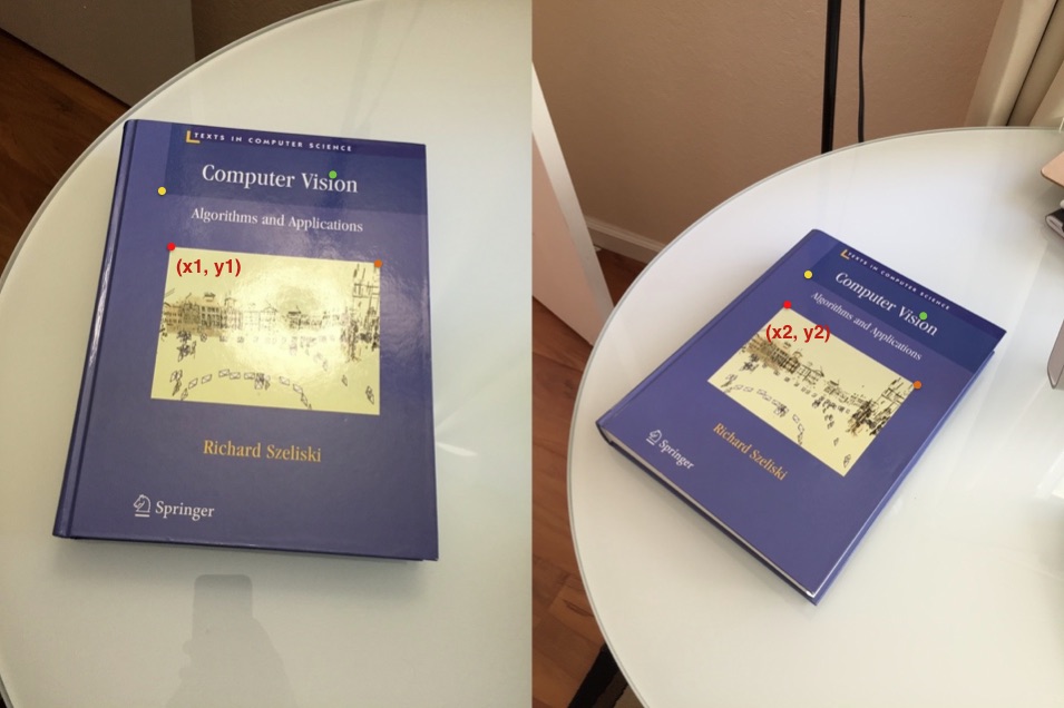
If we know 4 or more corresponding points in the two images, we can use the OpenCV function findHomography to find the homography. An example of four corresponding points is shown in the Figure above. The red, green, yellow and orange points are corresponding points.
Internally the function findHomography solves a linear system of equations to find the homography, but in this post we will not go over that math.
Let’s check the usage.

C++
findHomography(points1, points2, h)
Python
h, status = cv2.findHomography(points1, points2)
where, points1 and points2 are vectors/arrays of corresponding points, and h is the homography matrix.
How to find corresponding points automatically ?
In many Computer Vision applications, we often need to identify interesting stable points in an image. These points are called keypoints or feature points. There are several keypoint detectors implemented in OpenCV ( e.g. SIFT, SURF, and ORB).
In this tutorial, we will use the ORB feature detector because it was co-invented by my former labmate Vincent Rabaud. Just kidding! We will use ORB because SIFT and SURF are patented and if you want to use it in a real-world application, you need to pay a licensing fee. ORB is fast, accurate and license-free!
ORB keypoints are shown in the image below using circles.
ORB stands for Oriented FAST and Rotated BRIEF. Let’s see what FAST and BRIEF mean.
A feature point detector has two parts
- Locator: This identifies points on the image that are stable under image transformations like translation (shift), scale (increase / decrease in size), and rotation. The locator finds the x, y coordinates of such points. The locator used by the ORB detector is called FAST.
- Descriptor: The locator in the above step only tells us where the interesting points are. The second part of the feature detector is the descriptor which encodes the appearance of the point so that we can tell one feature point from the other. The descriptor evaluated at a feature point is simply an array of numbers. Ideally, the same physical point in two images should have the same descriptor. ORB uses a modified version of the feature descriptor called BRISK.
Note: In many applications in Computer Vision, we solve a recognition problem in two steps — a) Localization 2) Recognition.
For example, for implementing a face recognition system, we first need a face detector that outputs the coordinate of a rectangle inside which a face is located. The detector does not know or care who the person is. Its only job is to locate a face.
The second part of the system is a recognition algorithm. The original image is cropped to the detected face rectangle, and this cropped image is fed to the face recognition algorithm which ultimately recognizes the person. The locator of the feature detector acts like a face detector. It localizes interesting points but does not deal with the identity of the point. The descriptor describes the region around the point so it can be identified again in a different image.
The homography that relates the two images can be calculated only if we know corresponding features in the two images. So a matching algorithm is used to find which features in one image match features in the other image. For this purpose, the descriptor of every feature in one image is compared to the descriptor of every feature in the second image to find good matches.
OpenCV Image Alignment Code
In this section, we present C++ and Python code for image alignment using OpenCV. The entire code is present in the next section, but if you prefer to obtain all images and code, download using the link below.
Steps for Feature Based Image Alignment
Now we are in a position to summarize the steps involved in image alignment. The description below refers to the code in the next sections.
- Read Images : We first read the reference image (or the template image) and the image we want to align to this template in Lines 70-80 in C++ and Lines 56-65 in the Python code.
- Detect Features: We then detect ORB features in the two images. Although we need only 4 features to compute the homography, typically hundreds of features are detected in the two images. We control the number of features using the parameter MAX_FEATURES in the Python and C++ code. Lines 26-29 in the C++ code and Lines 16-19 in the Python code detect features and compute the descriptors using detectAndCompute.
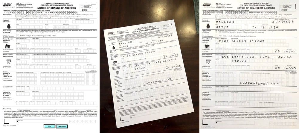
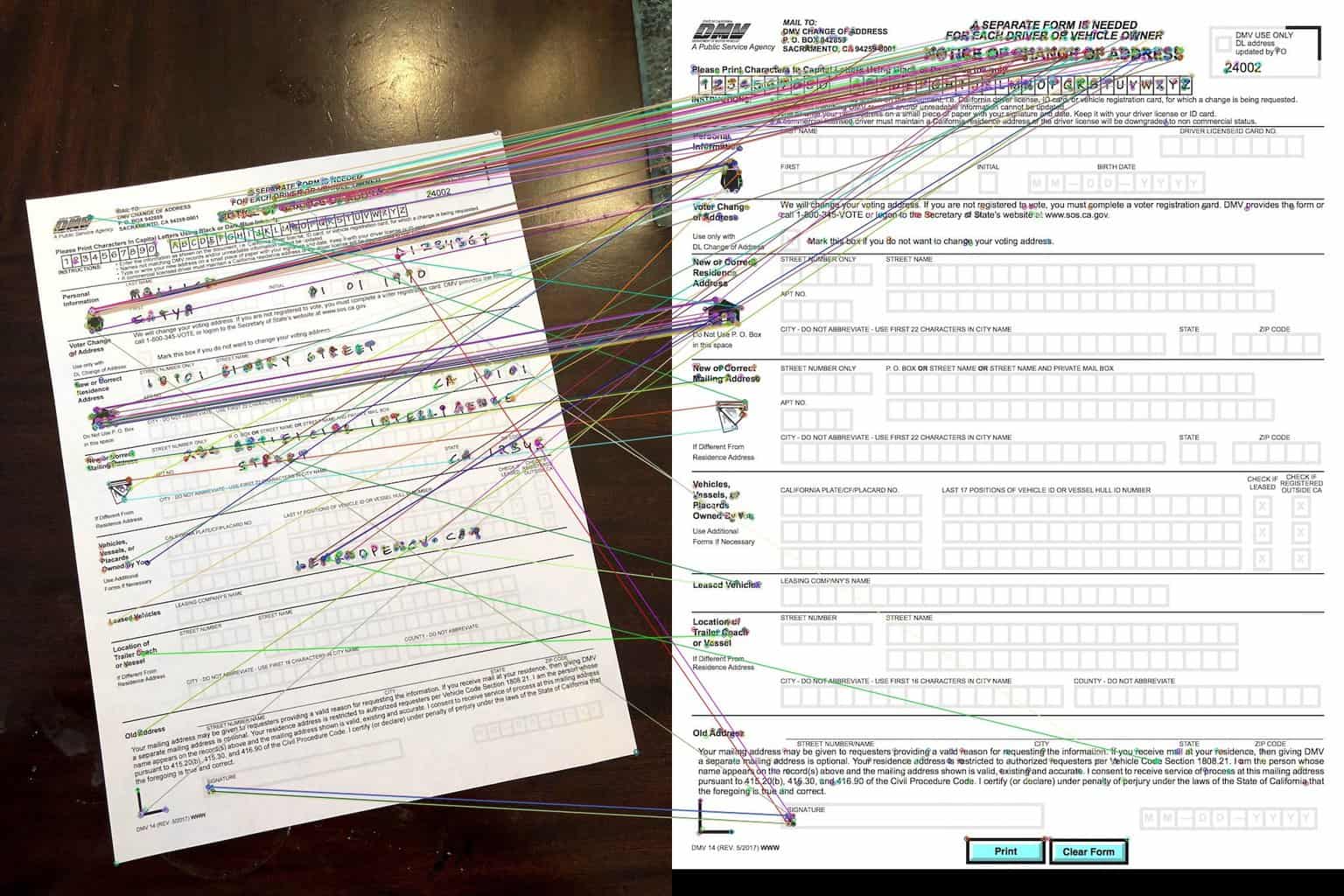
- Match Features: In Lines 31-47 in C++ and in Lines 21-34 in Python we find the matching features in the two images, sort them by goodness of match and keep only a small percentage of original matches. We finally display the good matches on the images and write the file to disk for visual inspection. We use the hamming distance as a measure of similarity between two feature descriptors. The matched features are shown in the figure below by drawing a line connecting them. Notice, we have many incorrect matches and thefore we will need to use a robust method to calculate homography in the next step.
C++ Code for Image Registration
#include <opencv2/opencv.hpp>
#include "opencv2/xfeatures2d.hpp"
#include "opencv2/features2d.hpp"

using namespace std;
using namespace cv;
using namespace cv::xfeatures2d;

const int MAX_FEATURES = 500;
const float GOOD_MATCH_PERCENT = 0.15f;

void alignImages(Mat &im1, Mat &im2, Mat &im1Reg, Mat &h)
{
  // Convert images to grayscale
  Mat im1Gray, im2Gray;
  cvtColor(im1, im1Gray, cv::COLOR_BGR2GRAY);
  cvtColor(im2, im2Gray, cv::COLOR_BGR2GRAY);

  // Variables to store keypoints and descriptors
  std::vector<KeyPoint> keypoints1, keypoints2;
  Mat descriptors1, descriptors2;

  // Detect ORB features and compute descriptors.
  Ptr<Feature2D> orb = ORB::create(MAX_FEATURES);
  orb->detectAndCompute(im1Gray, Mat(), keypoints1, descriptors1);
  orb->detectAndCompute(im2Gray, Mat(), keypoints2, descriptors2);

  // Match features.
  std::vector<DMatch> matches;
  Ptr<DescriptorMatcher> matcher = DescriptorMatcher::create("BruteForce-Hamming");
  matcher->match(descriptors1, descriptors2, matches, Mat());

  // Sort matches by score
  std::sort(matches.begin(), matches.end());

  // Remove not so good matches
  const int numGoodMatches = matches.size() * GOOD_MATCH_PERCENT;
  matches.erase(matches.begin()+numGoodMatches, matches.end());

  // Draw top matches
  Mat imMatches;
  drawMatches(im1, keypoints1, im2, keypoints2, matches, imMatches);
  imwrite("matches.jpg", imMatches);

  // Extract location of good matches
  std::vector<Point2f> points1, points2;

  for( size_t i = 0; i < matches.size(); i++ )
  {
    points1.push_back( keypoints1[ matches[i].queryIdx ].pt );
    points2.push_back( keypoints2[ matches[i].trainIdx ].pt );
  }

  // Find homography
  h = findHomography( points1, points2, RANSAC );

  // Use homography to warp image
  warpPerspective(im1, im1Reg, h, im2.size());
}

int main(int argc, char **argv)
{
  // Read reference image
  string refFilename("form.jpg");
  cout << "Reading reference image : " << refFilename << endl;
  Mat imReference = imread(refFilename);

  // Read image to be aligned
  string imFilename("scanned-form.jpg");
  cout << "Reading image to align : " << imFilename << endl;
  Mat im = imread(imFilename);

  // Registered image will be resotred in imReg.
  // The estimated homography will be stored in h.
  Mat imReg, h;

  // Align images
  cout << "Aligning images ..." << endl;
  alignImages(im, imReference, imReg, h);

  // Write aligned image to disk.
  string outFilename("aligned.jpg");
  cout << "Saving aligned image : " << outFilename << endl;
  imwrite(outFilename, imReg);

  // Print estimated homography
  cout << "Estimated homography : \n" << h << endl;
}
Python Code for Image Registration
from __future__ import print_function
import cv2
import numpy as np

MAX_FEATURES = 500
GOOD_MATCH_PERCENT = 0.15

def alignImages(im1, im2):

  # Convert images to grayscale
  im1Gray = cv2.cvtColor(im1, cv2.COLOR_BGR2GRAY)
  im2Gray = cv2.cvtColor(im2, cv2.COLOR_BGR2GRAY)

  # Detect ORB features and compute descriptors.
  orb = cv2.ORB_create(MAX_FEATURES)
  keypoints1, descriptors1 = orb.detectAndCompute(im1Gray, None)
  keypoints2, descriptors2 = orb.detectAndCompute(im2Gray, None)

  # Match features.
  matcher = cv2.DescriptorMatcher_create(cv2.DESCRIPTOR_MATCHER_BRUTEFORCE_HAMMING)
  matches = matcher.match(descriptors1, descriptors2, None)

  # Sort matches by score
  matches.sort(key=lambda x: x.distance, reverse=False)

  # Remove not so good matches
  numGoodMatches = int(len(matches) * GOOD_MATCH_PERCENT)
  matches = matches[:numGoodMatches]

  # Draw top matches
  imMatches = cv2.drawMatches(im1, keypoints1, im2, keypoints2, matches, None)
  cv2.imwrite("matches.jpg", imMatches)

  # Extract location of good matches
  points1 = np.zeros((len(matches), 2), dtype=np.float32)
  points2 = np.zeros((len(matches), 2), dtype=np.float32)

  for i, match in enumerate(matches):
    points1[i, :] = keypoints1[match.queryIdx].pt
    points2[i, :] = keypoints2[match.trainIdx].pt

  # Find homography
  h, mask = cv2.findHomography(points1, points2, cv2.RANSAC)

  # Use homography
  height, width, channels = im2.shape
  im1Reg = cv2.warpPerspective(im1, h, (width, height))

  return im1Reg, h

if __name__ == '__main__':

  # Read reference image
  refFilename = "form.jpg"
  print("Reading reference image : ", refFilename)
  imReference = cv2.imread(refFilename, cv2.IMREAD_COLOR)

  # Read image to be aligned
  imFilename = "scanned-form.jpg"
  print("Reading image to align : ", imFilename);
  im = cv2.imread(imFilename, cv2.IMREAD_COLOR)

  print("Aligning images ...")
  # Registered image will be resotred in imReg.
  # The estimated homography will be stored in h.
  imReg, h = alignImages(im, imReference)

  # Write aligned image to disk.
  outFilename = "aligned.jpg"
  print("Saving aligned image : ", outFilename);
  cv2.imwrite(outFilename, imReg)

  # Print estimated homography
  print("Estimated homography : \n",  h)
Summary
In this article we discussed how to perform feature-based image alignment using OpenCV. We started off with explaining the basic theory behind Homography. Then we went on to demonstrate the steps by way of an example in which we aligned a photo of a form taken using a mobile phone to a template of the form.
Subscribe & Download Code
If you liked this article and would like to download code (C++ and Python) and example images used in this post, please click here. Alternately, sign up to receive a free Computer Vision Resource Guide. In our newsletter, we share OpenCV tutorials and examples written in C++/Python, and Computer Vision and Machine Learning algorithms and news.Key Takeaways
- Image alignment (also called image registration) is the technique of warping one image ( or sometimes both images ) so that the features in the two images line up perfectly.
- Some interesting applications of Image Alignment are:
- Creating panoramas.
- In document processing applications, a good first step would be to align the scanned or photographed document to a template.
- Few medical applications where multiple scans of a tissue may be taken at slightly different times, and the two images are registered using a combination of techniques described in this tutorial and the previous one.
- The technique we used is often called “feature based” image alignment, a sparse set of features are detected in one image and matched with the features in the other image.
- A transformation is then calculated based on these matched features that warps one image on to the other.