This post is part of a series I am writing on Image Recognition and Object Detection.
The complete list of tutorials in this series is given below:
- Image recognition using traditional Computer Vision techniques : Part 1
- Histogram of Oriented Gradients : Part 2
- Example code for image recognition : Part 3
- Training a better eye detector: Part 4a
- Object detection using traditional Computer Vision techniques : Part 4b
- How to train and test your own OpenCV object detector : Part 5
- Image recognition using Deep Learning : Part 6
- Object detection using Deep Learning : Part 7
In this tutorial, we will build a simple handwritten digit classifier using OpenCV. As always we will share code written in C++ and Python.
This post is the third in a series I am writing on image recognition and object detection. The first post introduced the traditional computer vision image classification pipeline and in the second post, we discussed the Histogram of Oriented Gradients (HOG) image descriptor in detail. We also had a guest post on training an eye detector that is related to this topic.
The last two posts were geared toward providing education needed to understand the basics. This post is geared toward providing the training needed to successfully implement an image classifier. So, what is the difference between education and training ? Well, education provides largely theoretical knowledge. It is important to get that knowledge, but it is useless without good training. During training, you learn specific skills and apply the theoretical knowledge to the real world.
Image Classification Pipeline
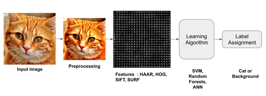
If you have not looked at my previous post on image classification, I encourage you to do so. In that post, a pipeline involved in most traditional computer vision image classification algorithms is described.
The image above shows that pipeline. In this post, we will use Histogram of Oriented Gradients as the feature descriptor and Support Vector Machine (SVM) as the machine learning algorithm for classification.
Optical Character Recognition (OCR) example using OpenCV (C++ / Python)
I wanted to share an example with code to demonstrate Image Classification using HOG + SVM. At the same time, I wanted to keep things as simple as possible so that we do not need much in addition to HOG and SVM. The inspiration and data for this post comes from the OpenCV tutorial here.
The original tutorial is in Python only, and for some strange reason implements it’s own simple HOG descriptor. We replaced their homegrown HOG with OpenCV’s HOG descriptor.
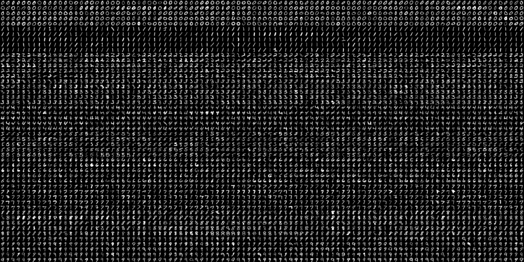
Digits dataset for OCR
We are going to use the above image as our dataset that comes with OpenCV samples. It contains 5000 images in all — 500 images of each digit. Each image is 20×20 grayscale with a black background. 4500 of these digits will be used for training and the remaining 500 will be used for testing the performance of the algorithm. You can click on the image above to enlarge.
Let us go through the steps needed to build and test a classifier.
Step 1 : Deskewing (Preprocessing)
People often think of a learning algorithm as a block box. Input an image at one end and out comes the result at the other end. In reality, you can assist the algorithm a bit and notice huge gains in performance. For example, if you are building a face recognition system, aligning the images to a reference face often leads to a quite substantial improvement in performance. A typical alignment operation uses a facial feature detector to align the eyes in every image.
Aligning digits before building a classifier similarly produces superior results. In the case of faces, aligment is rather obvious — you can apply a similarity transformation to an image of a face to align the two corners of the eyes to the two corners of a reference face.
In the case of handwritten digits, we do not have obvious features like the corners of the eyes we can use for alignment. However, an obvious variation in writing among people is the slant of their writing. Some writers have a right or forward slant where the digits are slanted forward, some have a backward or left slant, and some have no slant at all. We can help the algorithm quite a bit by fixing this vertical slant so it does not have to learn this variation of the digits. The image on the left shows the original digit in the first column and it’s deskewed (fixed) version.
This deskewing of simple grayscale images can be achieved using image moments. OpenCV has an implementation of moments and it comes in handy while calculating useful information like centroid, area, skewness of simple images with black backgrounds.
It turns out that a measure of the skewness is the given by the ratio of the two central moments ( mu11 / mu02 ). The skewness thus calculated can be used in calculating an affine transform that deskews the image.
The code for deskewing is shared below.
Python
def deskew(img):
m = cv2.moments(img)
if abs(m['mu02']) < 1e-2:
# no deskewing needed.
return img.copy()
# Calculate skew based on central momemts.
skew = m['mu11']/m['mu02']
# Calculate affine transform to correct skewness.
M = np.float32([[1, skew, -0.5*SZ*skew], [0, 1, 0]])
# Apply affine transform
img = cv2.warpAffine(img, M, (SZ, SZ), flags=cv2.WARP_INVERSE_MAP | cv2.INTER_LINEAR)
return img
C++
Mat deskew(Mat& img){
    Moments m = moments(img);
    if(abs(m.mu02) < 1e-2){
        return img.clone();
    }
    float skew = m.mu11/m.mu02;
    Mat warpMat = (Mat_<float>(2,3) << 1, skew, -0.5*SZ*skew, 0, 1, 0);
    Mat imgOut = Mat::zeros(img.rows, img.cols, img.type());
    warpAffine(img, imgOut, warpMat, imgOut.size(),affineFlags);

    return imgOut;
}
Step 2 : Calculate the Histogram of Oriented Gradients (HOG) descriptor
In this step, we will convert the grayscale image to a feature vector using the HOG feature descriptor. In my previous post, I had explained the HOG descriptor in great detail.
When I was in grad school, I found a huge gap between theory and practice. Acquiring the knowledge was easy. I could read papers and books. If I did not understand the concept or the math, I read more papers and books. That was the easy part. The hard part of putting that knowledge into practice. Part of the reason was that a lot of these algorithms worked after tedious handtuning and it was not obvious how to set the right parameters. For example, in Harris corner detector, why is the free parameter k set to 0.04 ? Why not 1 or 2 or 0.34212 instead? Why is 42 the answer to life, universe, and everything?
As I got more real world experience, I realized that in some cases you can make an educated guess but in other cases, nobody knows why. People often do a parameter sweep — they change different parameters in a principled way to see what produces the best result. Sometimes, the best parameters have an intuitive explanation and sometimes they don’t.
Keeping that in mind, let’s see what parameters were chosen for our HOG descriptor. We will also try to explain why they made sense, but instead of a rigorous proof, I will offer vigorous handwaving!
C++
HOGDescriptor hog(
Size(20,20), //winSize
Size(10,10), //blocksize
Size(5,5), //blockStride,
Size(10,10), //cellSize,
9, //nbins,
1, //derivAper,
-1, //winSigma,
0, //histogramNormType,
0.2, //L2HysThresh,
1,//gammal correction,
64,//nlevels=64
1);//Use signed gradients
Python
winSize = (20,20)
blockSize = (10,10)
blockStride = (5,5)
cellSize = (10,10)
nbins = 9
derivAperture = 1
winSigma = -1.
histogramNormType = 0
L2HysThreshold = 0.2
gammaCorrection = 1
nlevels = 64
signedGradients = True

hog = cv2.HOGDescriptor(winSize,blockSize,blockStride,
cellSize,nbins,derivAperture,
winSigma,histogramNormType,L2HysThreshold,
gammaCorrection,nlevels, useSignedGradients)
I am not going to describe derivAperture, winSigma, histogramNormType, L2HysThreshold, gammaCorrection and nlevels because I have never had to change these parameters while using the HOG descriptor. Unless you have carefully read the original HOG paper, I would recommend you go with the default values. Let’s explore the choice of other parameters.
winSize: This parameter is set to 20×20 because the size of the digit images in our dataset is 20×20 and we want to calculate one descriptor for the entire image.
cellSize: Our digits are 20×20 grayscale images. In other words, our image is represented by 20×20 = 400 numbers.The size of descriptor typically is much smaller than the number of pixels in an image. The cellSize is chosen based on the scale of the features important to do the classification. A very small cellSize would blow up the size of the feature vector and a very large one may not capture relevant information. You should test this yourself using the code shared in this post. We have chosen the cellSize of 10×10 in this tutorial. Could we have chosen 8 ? Yup, that would have worked too.
blockSize: The notion of blocks exist to tackle illumination variation. A large block size makes local changes less significant while a smaller block size weights local changes more. Typically blockSize is set to 2 x cellSize, but in our example of digits classification, illumination does not present much of a challenge. In my experiments, a blockSize of 10×10 gave the best results.
blockStride: The blockStride determines the overlap between neighboring blocks and controls the degree of contrast normalization. Typically a blockStride is set to 50% of blockSize.
nbins: nbins sets the number of bins in the histogram of gradients. The authors of the HOG paper had recommended a value of 9 to capture gradients between 0 and 180 degrees in 20 degrees increments. In my experiments, increasing this value to 18 did not produce any better results.
signedGradients: Typically gradients can have any orientation between 0 and 360 degrees. These gradients are referred to as “signed” gradients as opposed to “unsigned” gradients that drop the sign and take values between 0 and 180 degrees. In the original HOG paper, unsigned gradients were used for pedestrian detection. In my experiments, for this problem, signed gradients produced slightly better results.
The HOG descriptor defined above can be used to compute the HOG features of an image using the following code.
C++
// im is of type Mat
vector<float> descriptors;
hog.compute(im,descriptor);
Python
descriptor = hog.compute(im)
The size of this descriptor is 81×1 for the parameters we have chosen.
Step 3: Training a Model ( a.k.a Learning a Classifier )
Until this point, we have deskewed the original image and defined a descriptor for our image. This has allowed us to convert every image in our dataset to a vector of size 81×1.
We are now ready to train a model that will classify the images in our training set. To do this we have chosen Support Vector Machines (SVM) as our classification algorithm. While the theory and math behind SVM is involved and beyond the scope of this tutorial, how it works is very intuitive and easy to understand. You can check out my previous post that explains Linear SVMs.
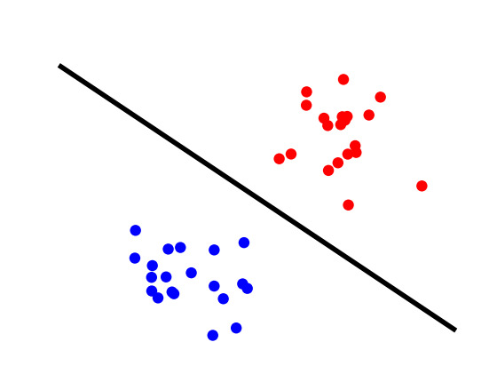
To quickly recap, if you have points in an n-dimensional space and class labels attached to the points, a Linear SVM will divide the space using planes such that different classes are on different sides of the plane. In the figure below, we have two classes represented by red and blue dots. If this data is fed into a Linear SVM, it will easily build a classifier by finding the line that clearly separates the two classes. There are many lines that could have separated this data. SVM chooses the one that is at a maximum distance data points of either class.
The two-class example shown in the figure above may appear simple compared to our digits classification problem, but mathematically they are very similar. Instead of being points in a 2D space, our images descriptors are points in an 81-dimensional space because they are represented by an 81×1 vector. The class labels attached to these points are the digits contained in the image, i.e. 0, 1, 2, … 9. Instead of lines in 2D, the SVM will find hyperplanes in a high dimensional space to do the classification.
SVM Parameter C
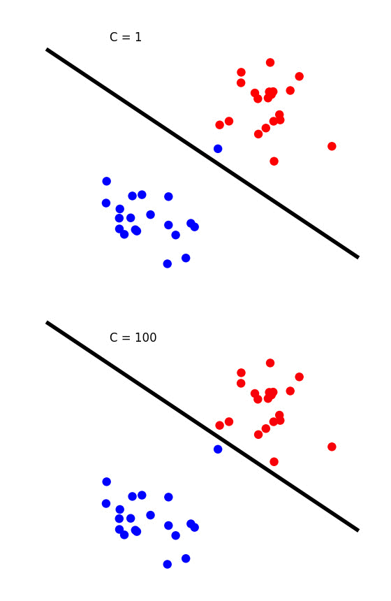
One of the two common parameters you need to know about while training an SVM is called C. Real world data is not as clean as shown above. Sometimes the training data may have mislabeled examples. At other times, one example of a set may be too close in appearance to another example. E.g. a handwritten digit 2 may look like a 3.
In the animation below we have created this scenario. Notice, the blue dot is too close to the red cluster. When the default value of C = 1 is chosen, the blue dot is misclassified. Choosing the value of 100 for C classifies it correctly.
But now the decision boundary represented by the black line is too close to one of the classes. Would you rather choose C to be 1 where one data point is misclassified, but the separation between the classes is much better ( minus the one data point )? The parameter C allows you to control this tradeoff.
So, how do you choose C? We choose the C that provides the best classification on a held out test set. The images in this set were not used in training.
SVM Parameter Gamma : Non-Linear SVM
Did you notice, I sneaked in the word “Linear” a few times? In classification tasks, a dataset consisting of many classes is called linearly separable if the space containing the data can be partitioned using planes ( or lines in 2D ) to separate the classes.
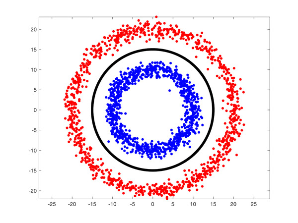
What if the data is not linearly separable? The figure below shows two classes using red and blue dots that are not linearly separable. You cannot draw a line on the plane to separate the two classes. A good classifier, represented using the black line, is more of a circle.
In real life, data is messy and not linearly separable.
Can we still use SVMs? The answer is YES!
To accomplish this, you use a technique called the Kernel Trick. It is a neat trick that transforms non-linearly separable data into a linearly separable one. In our example, the red and blue dots lie on a 2D plane. Let us add a third dimension to all data points using the following equation.
![]()
If you ever hear people using the fancy term Radial Basis Function (RBF) with a Gaussian Kernel, they are simply talking about the above equation. RBF is simply a real-valued function that depends only on the distance from the origin ( i.e. depends only on ![]() ). The Gaussian Kernel refers to the Gaussian form of the above equation. More generally, an RBF can have different kinds of kernels. You can see some of them here.
). The Gaussian Kernel refers to the Gaussian form of the above equation. More generally, an RBF can have different kinds of kernels. You can see some of them here.
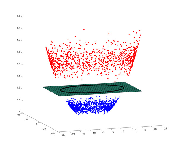
So, we just cooked up a third dimension based on data in the other two dimensions. The figure below shows this three-dimensional (x, y, z) data. We can see it is separable by the plane containing the black circle!
The parameter Gamma ( ![]() ) controls the stretching of data in the third dimension. It helps in classification but it also distorts the data. Like Goldilocks, you have to choose this parameter to be “just right”. It is one of the two important parameters people choose while training an SVM.
) controls the stretching of data in the third dimension. It helps in classification but it also distorts the data. Like Goldilocks, you have to choose this parameter to be “just right”. It is one of the two important parameters people choose while training an SVM.
Equipped with this knowledge, we are now ready to train an SVM using OpenCV.
Training and Testing an SVM using OpenCV
Under the hood, OpenCV uses LIBSVM. SVM in OpenCV 2.4.x still uses the C API. Fortunately, starting 3.x, OpenCV now uses the much nicer C++ API. Here is how you set up SVM using OpenCV in C++ and Python.
C++
// Set up SVM for OpenCV 3
Ptr<SVM> svm = SVM::create();
// Set SVM type
svm->setType(SVM::C_SVC);
// Set SVM Kernel to Radial Basis Function (RBF)
svm->setKernel(SVM::RBF);
// Set parameter C
svm->setC(12.5);
// Set parameter Gamma
svm->setGamma(0.50625);

// Train SVM on training data
Ptr<TrainData> td = TrainData::create(trainMat, ROW_SAMPLE, trainLabels);
svm->train(td);

// Save trained model
svm->save("digits_svm_model.yml");

// Test on a held out test set
svm->predict(testMat, testResponse);
Python
# Set up SVM for OpenCV 3
svm = cv2.ml.SVM_create()
# Set SVM type
svm.setType(cv2.ml.SVM_C_SVC)
# Set SVM Kernel to Radial Basis Function (RBF)
svm.setKernel(cv2.ml.SVM_RBF)
# Set parameter C
svm.setC(C)
# Set parameter Gamma
svm.setGamma(gamma)

# Train SVM on training data
svm.train(trainData, cv2.ml.ROW_SAMPLE, trainLabels)

# Save trained model
svm->save("digits_svm_model.yml");

# Test on a held out test set
testResponse = svm.predict(testData)[1].ravel()
Auto Training SVM
As you can imagine, it can be very time consuming to select the right SVM parameters C and Gamma. Fortunately, OpenCV 3.x C++ API provides a function that automatically does this hyperparameter optimization for you and provides the best C and Gamma values. In the code above, you can change svm->train(td) to the following
svm->trainAuto(td);
This training can take a very long time ( say 5x more than svm->train ) because it is essentially training multiple times.
OpenCV SVM bugs
We encountered two bugs while working with OpenCV SVM. The first one is confirmed, but the other two are not.
- SVM model won’t load in Python API. The trained SVM model you just saved won’t load if you are using Python! Is the bug fix coming ? Nope! Check it out here
- trainAuto does not appear to be exposed via the Python API.
- SVM with RBF kernel does not work in iOS / Android. I would be happy to be proven wrong, but on mobile platforms ( iOS / Android ), we have not been able to use the SVM trained with RBF kernel. The SVM response is always the same. Linear SVM models work just fine.
Results
After training and some hyperparameter optimization, we hit 98.6% on digits classification! Not, bad for just a few seconds of training.
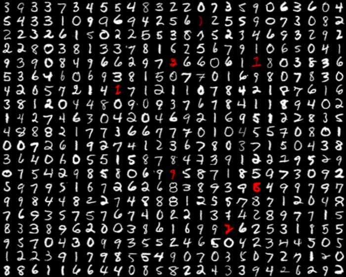
Out of the 500 images in the training set, 7 were misclassified. The images and their misclassified labels are shown below. Like a father looking at his kid’s mistake, I would say these mistakes are understandable.










100K+ Learners
Join Free OpenCV Bootcamp3 Hours of Learning