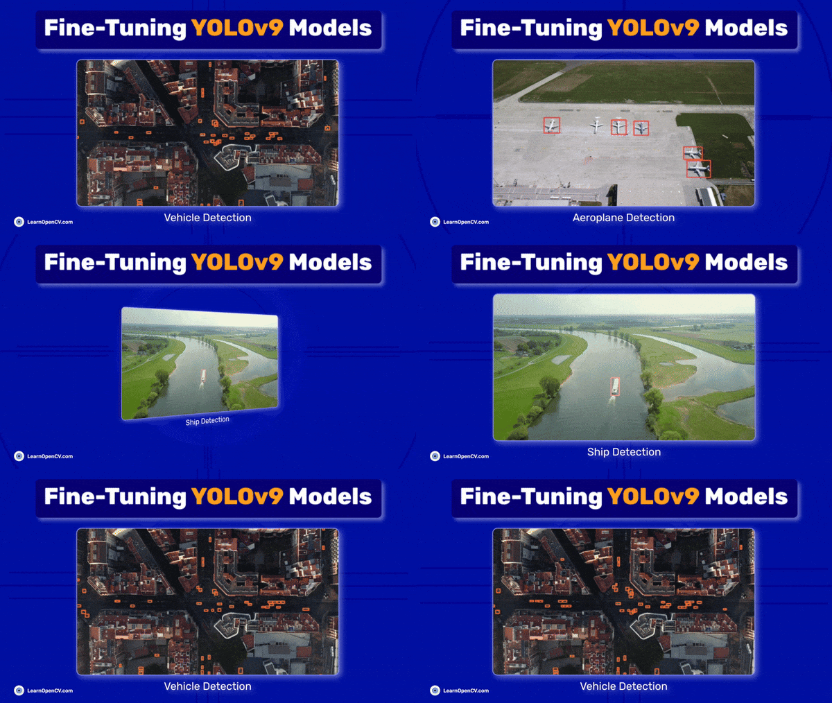
Fine-Tuning YOLOv9 Models on Custom Dataset

Fine-tuning YOLOv9 models on custom datasets can dramatically enhance object detection performance, but how significant is this improvement? In this comprehensive exploration, YOLOv9 has been fine-tuned on the SkyFusion dataset, with three distinct classes: aircraft, ship, and vehicle. Through an extensive series of experiments, including modifications to learning rates, image sizes, and strategic freezing of the backbone, an impressive mAP50 value of 0.766 has been achieved!

This research article not only details these significant results but also provides access to the fine-tuning code behind these experiments. SCROLL BELOW to the concluding part of the article or click here to see the experimental results right away.

What’s New With YOLOv9 and GELAN?

Before trying to get into more detail about GELAN, it is better to understand the importance of the ELAN approach.

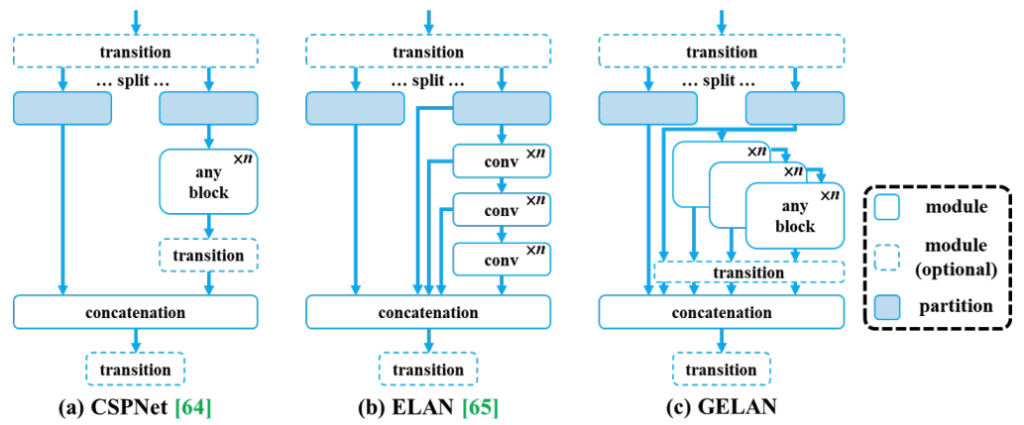
In the research paper by Chien-Yao Wang et al., [1] the architecture of Efficient Layer Aggregation Network (or) ELAN has been proposed. This ELAN represents a sophisticated approach in the domain of gradient path designed networks, specifically tailored to address the diminishing returns in model convergence during scaling. Central to ELAN’s design philosophy is the optimization of gradient propagation paths through meticulous analysis of both the shortest and longest gradient paths across the network’s layers.

This innovative architecture synergizes the robustness of VoVNet with the efficiency of CSPNet, further enhancing gradient flow via a unique structural element known as the stack in the computational block. This component strategically mitigates the adverse effects of depth-induced convergence deterioration, a common pitfall observed in scaling models like scaled YOLOv4. ELAN’s design significantly counters the diminishing accuracy gains and potential convergence issues associated with excessive depth, as evidenced by comparative analysis against traditional architectures like ResNet and VoVNet, underscoring its superior performance in maintaining effective gradient flow even as the network depth increases.

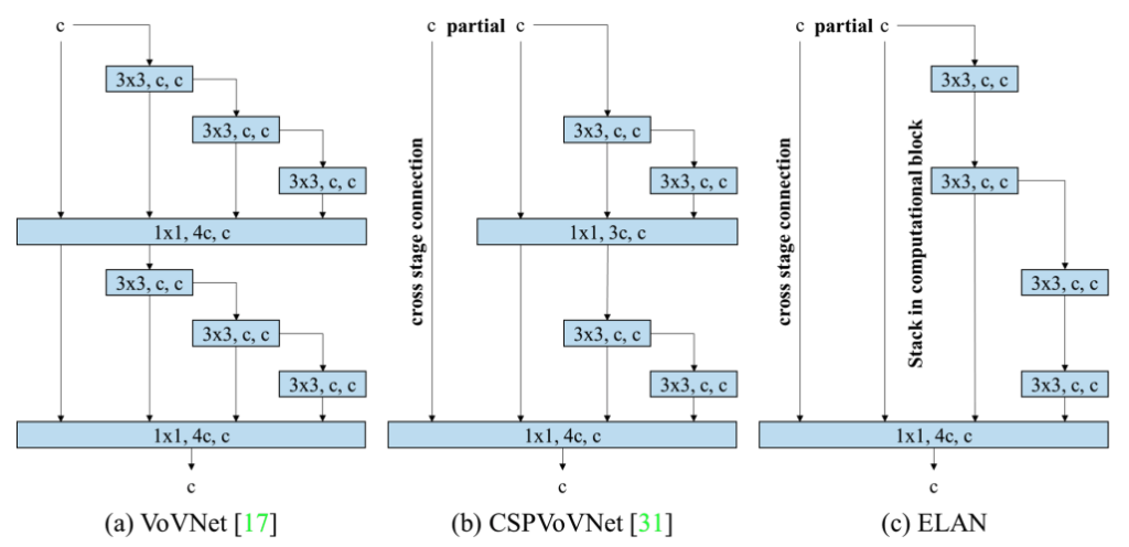
In the YOLOv9 research paper by Chien-Yao Wang, I-Hau Yeh, and Hong-Yuan Mark Liao [2], the Generalized Efficient Layer Aggregation Network (GELAN) has been proposed. It represents a pioneering advancement in network architecture by integrating the foundational principles of CSPNet and ELAN, aiming to optimize gradient path planning. This novel architecture is designed to enhance model performance across key metrics: lightweight design, inference speed, and accuracy. GELAN expands upon ELAN’s original framework, which primarily focused on stacking convolutional layers, evolving into a versatile structure capable of incorporating a variety of computational blocks.

Model Architecture: YOLOv9-C & YOLOv9-E

Given below is the overall network architecture of the YOLOv9-C model:

backbone:
  - [-1, 1, Conv, [64, 3, 2]]  # 0-P1/2
  - [-1, 1, Conv, [128, 3, 2]]  # 1-P2/4
  - [-1, 1, RepNCSPELAN4, [256, 128, 64, 1]]  # 2
  - [-1, 1, ADown, [256]]  # 3-P3/8
  - [-1, 1, RepNCSPELAN4, [512, 256, 128, 1]]  # 4
  - [-1, 1, ADown, [512]]  # 5-P4/16
  - [-1, 1, RepNCSPELAN4, [512, 512, 256, 1]]  # 6
  - [-1, 1, ADown, [512]]  # 7-P5/32
  - [-1, 1, RepNCSPELAN4, [512, 512, 256, 1]]  # 8
  - [-1, 1, SPPELAN, [512, 256]]  # 9

head:
  - [-1, 1, nn.Upsample, [None, 2, 'nearest']]
  - [[-1, 6], 1, Concat, [1]]  # cat backbone P4
  - [-1, 1, RepNCSPELAN4, [512, 512, 256, 1]]  # 12

  - [-1, 1, nn.Upsample, [None, 2, 'nearest']]
  - [[-1, 4], 1, Concat, [1]]  # cat backbone P3
  - [-1, 1, RepNCSPELAN4, [256, 256, 128, 1]]  # 15 (P3/8-small)

  - [-1, 1, ADown, [256]]
  - [[-1, 12], 1, Concat, [1]]  # cat head P4
  - [-1, 1, RepNCSPELAN4, [512, 512, 256, 1]]  # 18 (P4/16-medium)

  - [-1, 1, ADown, [512]]
  - [[-1, 9], 1, Concat, [1]]  # cat head P5
  - [-1, 1, RepNCSPELAN4, [512, 512, 256, 1]]  # 21 (P5/32-large)

  - [[15, 18, 21], 1, Detect, [nc]]  # DDetect(P3, P4, P5)

Highlights

• YOLOv9-C employs a strategic layering of RepNCSPELAN4 and ADown blocks, boosting feature extraction efficiency and expanding the receptive field without sacrificing computational speed.
• The architecture’s use of upsampling and concatenation in the head section enriches feature integration, enabling nuanced multi-scale detection across varied object sizes.
• With the integrated Detect layer, YOLOv9-C adeptly gets features from multiple depths, showcasing its robustness in accurately detecting objects across a spectrum of scales.

The backbone structure begins with consecutive convolutional layers, incrementally doubling the channels from 64 to 512, facilitating initial feature extraction at varying scales (P1/2 to P5/32). At the core of this architecture are RepNCSPELAN4 blocks, which are recurrent layers integrating NCSPELAN (Nested CSP-Efficient Layer Aggregation Network) units, tailored for efficient gradient flow and feature integration across the network depth.

The model employs alternate layers of RepNCSPELAN4 and adaptive down-sampling (ADown), systematically expanding the receptive field while maintaining computational efficiency. In the head section, the architecture uses upsampling and concatenation operations to merge features from different backbone levels, enhancing feature richness for the detection task. This multi-scale approach, evident in the concatenation of feature maps from various depths, ensures a comprehensive feature representation at three critical scales, optimizing the model for detecting objects of varying sizes.

In the end, the integrated Detect layer amalgamates the multi-level features to output the final detection results, indicating the model’s capacity to handle diverse object scales effectively.

Given below is the overall network architecture of the YOLOv9-E model:

backbone:
  - [-1, 1, Silence, []]
  - [-1, 1, Conv, [64, 3, 2]]  # 1-P1/2
  - [-1, 1, Conv, [128, 3, 2]]  # 2-P2/4
  - [-1, 1, RepNCSPELAN4, [256, 128, 64, 2]]  # 3
  - [-1, 1, ADown, [256]]  # 4-P3/8
  - [-1, 1, RepNCSPELAN4, [512, 256, 128, 2]]  # 5
  - [-1, 1, ADown, [512]]  # 6-P4/16
  - [-1, 1, RepNCSPELAN4, [1024, 512, 256, 2]]  # 7
  - [-1, 1, ADown, [1024]]  # 8-P5/32
  - [-1, 1, RepNCSPELAN4, [1024, 512, 256, 2]]  # 9
   
  - [1, 1, CBLinear, [[64]]] # 10
  - [3, 1, CBLinear, [[64, 128]]] # 11
  - [5, 1, CBLinear, [[64, 128, 256]]] # 12
  - [7, 1, CBLinear, [[64, 128, 256, 512]]] # 13
  - [9, 1, CBLinear, [[64, 128, 256, 512, 1024]]] # 14
  
  - [0, 1, Conv, [64, 3, 2]]  # 15-P1/2
  - [[10, 11, 12, 13, 14, -1], 1, CBFuse, [[0, 0, 0, 0, 0]]] # 16
  - [-1, 1, Conv, [128, 3, 2]]  # 17-P2/4
  - [[11, 12, 13, 14, -1], 1, CBFuse, [[1, 1, 1, 1]]] # 18  
  - [-1, 1, RepNCSPELAN4, [256, 128, 64, 2]]  # 19
  - [-1, 1, ADown, [256]]  # 20-P3/8
  - [[12, 13, 14, -1], 1, CBFuse, [[2, 2, 2]]] # 21  
  - [-1, 1, RepNCSPELAN4, [512, 256, 128, 2]]  # 22
  - [-1, 1, ADown, [512]]  # 23-P4/16
  - [[13, 14, -1], 1, CBFuse, [[3, 3]]] # 24 
  - [-1, 1, RepNCSPELAN4, [1024, 512, 256, 2]]  # 25
  - [-1, 1, ADown, [1024]]  # 26-P5/32
  - [[14, -1], 1, CBFuse, [[4]]] # 27
  - [-1, 1, RepNCSPELAN4, [1024, 512, 256, 2]]  # 28
  - [-1, 1, SPPELAN, [512, 256]]  # 29

head:
  - [-1, 1, nn.Upsample, [None, 2, 'nearest']]
  - [[-1, 25], 1, Concat, [1]]  # cat backbone P4
  - [-1, 1, RepNCSPELAN4, [512, 512, 256, 2]]  # 32

  - [-1, 1, nn.Upsample, [None, 2, 'nearest']]
  - [[-1, 22], 1, Concat, [1]]  # cat backbone P3
  - [-1, 1, RepNCSPELAN4, [256, 256, 128, 2]]  # 35 (P3/8-small)

  - [-1, 1, ADown, [256]]
  - [[-1, 32], 1, Concat, [1]]  # cat head P4
  - [-1, 1, RepNCSPELAN4, [512, 512, 256, 2]]  # 38 (P4/16-medium)

  - [-1, 1, ADown, [512]]
  - [[-1, 29], 1, Concat, [1]]  # cat head P5
  - [-1, 1, RepNCSPELAN4, [512, 1024, 512, 2]]  # 41 (P5/32-large)

   # detect
  - [[35, 38, 41], 1, Detect, [nc]]  # Detect(P3, P4, P5)

On the other hand, the YOLOv9-E model is a bigger model than YOLOv9-C in-terms of total number of blocks and layers. Let’s have a look at this as well.

Highlights

• YOLOv9-E augments the network’s depth and complexity with Silence and CBLinear layers, enhancing channel-wise feature optimization and significantly increasing the channel capacity up to 1024.
• This variant employs CBFuse layers for advanced feature fusion across varying depths, offering a more intricate and effective feature integration compared to YOLOv9-C.
• YOLOv9-E maintains detailed and high-resolution feature extraction at greater depths, supported by the strategic use of RepNCSPELAN4, ADown, and SPPELAN layers, ensuring superior performance in complex object detection tasks.

Unlike YOLOv9-C, YOLOv9-E introduces the ‘Silence’ and CBLinear layers, indicating a strategic silence operation and linear combination of channel-wise features to optimize depth and complexity. This model increases the use of RepNCSPELAN4 blocks across deeper network layers, employing a higher repetition and wider channel spectrum, culminating in 1024 channels, thus enhancing feature extraction and representation.

The integration of ‘CBFuse’ layers signifies a novel approach in YOLOv9-E, facilitating the fusion of features across different network depths, which contrasts with the more straightforward concatenation and upsampling in YOLOv9-C. This sophisticated fusion strategy ensures richer, more diversified feature integration, optimizing the model for complex detection scenarios. The strategic placement of adaptive down-sampling (ADown) and SPPELAN layers further refines the feature processing, ensuring that YOLOv9-E maintains high resolution and detailed feature extraction even at increased network depths.

SkyFusion: Dataset Visualization

In this research article, the SkyFusion Aerial Object Detection dataset has been used for fine-tuning YOLOv9 models. Let’s have a look at a few samples from this dataset as well.

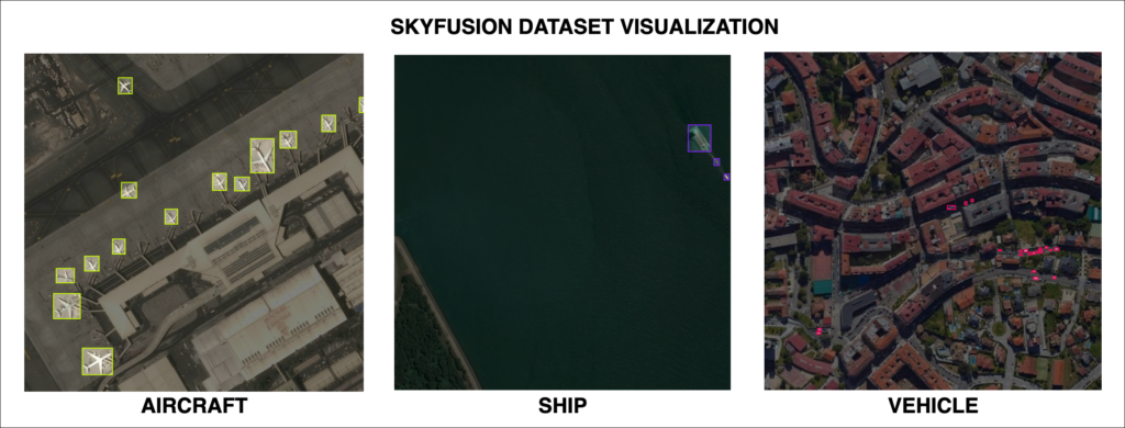
As shown in FIGURE 3, the dataset has three classes, namely: Aircraft, Ship and Vehicle. It was created by fusing the AITODv2 and Airbus Aircraft Detection datasets. The specifications are shown below: 

• Train: 2095 images
• Test: 450 images
• Valid: 450 images

Hence, this dataset contains 2995 images in total.

Click here to download the source code to this post

Code Walkthrough

In this section, we can go ahead and understand the setup process for Ultralytics YOLOv9 models. Parallely, you can also download the notebook used in this research work.

Initially, the Ultralytics package needs to be installed in your development environment. For that, the following command can be used:

!pip install ultralytics

Since, this is an ultralytics based training procedure, everything can be done with just 2-3 lines of code itself.

Let’s import the ultralytics package using this command: 

from ultralytics import YOLO

Next, let’s import the YOLOv9 model of choice using this:

model = YOLO('yolov9c.pt')

This above line of code imports the YOLOv9-C model, and downloads the pretrained weights from ultralytics’ repository, into your local environment.

From here, we can start the training procedure: 

results=model.train(data=’path_to_dataset_yaml’, epochs=’no_of_epochs’, imgsz=’image_size’, batch=’batch_size’)

That’s it, this is all you need to get this model up and ready for training!

Baseline Training Performance Metrics – YOLOv9-C and YOLOv9-E

Alright, so how do these models perform without any type of fine-tuning? Let’s have a look at the baseline results.

In this initial experiment, the YOLOv9-C model was used to train for 100 EPOCHS with a batch size of 16. In the 100th EPOCH it reached a mAP50 value of 0.712. The training graphs for this experiment are shown below:

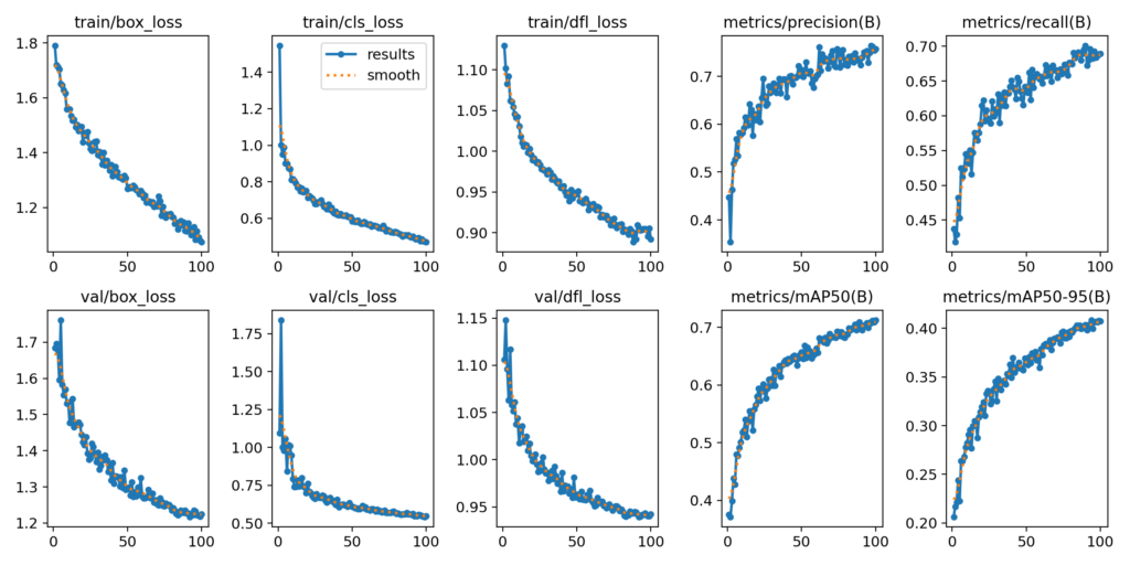
From the graphical visualization shown above, it can be seen that this YOLOv9-C model is able to reach an mAP50 value of 0.516 in just 10 EPOCHS. This is great!

But can this model do better? Let’s try training the same model for more epochs. Hence, the YOLOv9-C model was trained for 150 EPOCHS to check if it can cross the mAP50 value of 0.712 from the previous run.

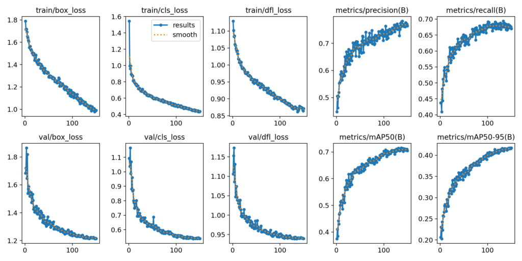
By increasing the number of training epochs, we were also able to improve the mAP50 metric from 0.754 to 0.766.

From these two experiments, we’ve had a chance to understand what YOLOv9 models are capable of, even without any kind of fine-tuning. But, is it any better than the baseline performance results from the evergreen YOLOv8 model?

In this experimental run, the YOLOv8-M model was trained on the same SkyFusion dataset for 100 EPOCHS. Here are the results:

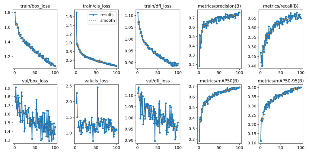
From these results, it has been observed that the YOLOv8-M model achieves 0.689 mAP50 compared to 0.71 mAP50 on the YOLOv9-C model. This clearly indicates the difference in performance between the new YOLOv9 models and the older YOLOv8 models. So far, we’ve just tried to train the models as they are without making any hyperparameter changes.

Fine-Tuning YOLOv9 Models – A Model Centric Approach

The earlier sections examined these YOLOv9 models without any fine-tuning. Let’s go ahead and explore techniques for fine-tuning YOLOv9 models with a series of experiments that showcase different techniques to do just that.

NOTE: All the runs shown in this research article were done on an Nvidia RTX A6000 GPU with 48GB GDDR6 vRAM.

Experiment 1: Freezing the Backbone + Lower Learning Rate at 0.001

Before we proceed, let’s have a look at the YOLOv9-C model’s internal architecture once again:

backbone:
  - [-1, 1, Conv, [64, 3, 2]]  # 0-P1/2
  - [-1, 1, Conv, [128, 3, 2]]  # 1-P2/4
  - [-1, 1, RepNCSPELAN4, [256, 128, 64, 1]]  # 2
  - [-1, 1, ADown, [256]]  # 3-P3/8
  - [-1, 1, RepNCSPELAN4, [512, 256, 128, 1]]  # 4
  - [-1, 1, ADown, [512]]  # 5-P4/16
  - [-1, 1, RepNCSPELAN4, [512, 512, 256, 1]]  # 6
  - [-1, 1, ADown, [512]]  # 7-P5/32
  - [-1, 1, RepNCSPELAN4, [512, 512, 256, 1]]  # 8
  - [-1, 1, SPPELAN, [512, 256]]  # 9

head:
  - [-1, 1, nn.Upsample, [None, 2, 'nearest']]
  - [[-1, 6], 1, Concat, [1]]  # cat backbone P4
  - [-1, 1, RepNCSPELAN4, [512, 512, 256, 1]]  # 12

  - [-1, 1, nn.Upsample, [None, 2, 'nearest']]
  - [[-1, 4], 1, Concat, [1]]  # cat backbone P3
  - [-1, 1, RepNCSPELAN4, [256, 256, 128, 1]]  # 15 (P3/8-small)

  - [-1, 1, ADown, [256]]
  - [[-1, 12], 1, Concat, [1]]  # cat head P4
  - [-1, 1, RepNCSPELAN4, [512, 512, 256, 1]]  # 18 (P4/16-medium)

  - [-1, 1, ADown, [512]]
  - [[-1, 9], 1, Concat, [1]]  # cat head P5
  - [-1, 1, RepNCSPELAN4, [512, 512, 256, 1]]  # 21 (P5/32-large)

  - [[15, 18, 21], 1, Detect, [nc]]  # DDetect(P3, P4, P5)

From the model architecture shown above, it can be observed that the first 10 layers from 0-9 represent the layers that are part of the GELAN backbone. Let’s freeze them and see how it trains, shall we?

But the thing is, since we now have fewer layers, it’s better to train with a lesser learning rate. To carry out this, the default learning rate, i.e.  lr0=0.01 has been updated to lr0=0.001. To run this specific experiment, the following line of code can be used:

results = model.train(data='SkyFusion-YOLOv9/data.yaml', epochs=100, imgsz=640, batch=16, freeze=10, lr0=0.001, workers=0)

NOTE: Sometimes, while freezing the backbone on ultralytics you might get this ‘RuntimeError: CUDA error: OS call failed or operation not supported on this OS` came up. To fix this, the official PyTorch documentation asks to set the num_workers = 0, as CUDA tensors cannot perform multiprocessing, at least as of 11.03.2023. This will make the training process really slow, but it works. This article will be updated as soon as there is a fix.

Here are the results from Experiment 1: 

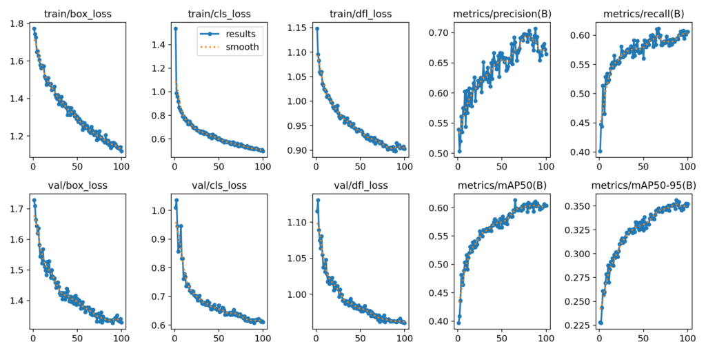
The results show that this experiment achieved an mAP50 value of 0.609, which is less than the full baseline. This can be explained by the lower learning rate of lr0=0.001 used in this experiment.

Experiment 2: Freezing Backbone + Learning Rate at 0.01

In this experiment, let’s roll back to the default learning rate of 0.01 and initialize the training process.

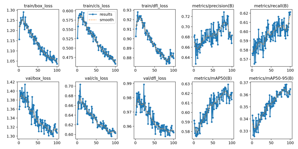
This setup has increased the mAP50 value to 0.629 from 0.609 in the previous experiment. But can we achieve any better results?

Experiment 3: Freezing Backbone + Enlarged Input Image Size

In the previous experiments, just the backbone alone was frozen. Even the learning rate was tweaked from 0.01 to see if there were any changes in mAP50 value. And as a matter of fact, there was indeed an improvement.

Moving forward – In this experiment, along with the frozen backbone, a larger input image size of 1024 was used. Let’s stick with lr0=0.01 and change the imgsz=1024 param, with the batch size as 8. Another point to consider is that this experiment might help with the detection of small objects, which is actually the case with this dataset.

The training code can be tweaked in the following way:

results = model.train(data='SkyFusion-YOLOv9/data.yaml', epochs=100, imgsz=1024, batch=4, freeze=10, workers=0)

Here are the results from this experiment: 

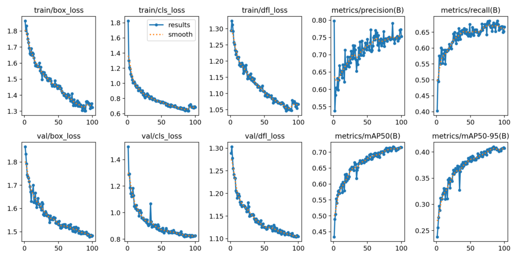
It turns out that there is an improvement after enlarging the image size and the learning rate. This was able to yield an mAP50 value of 0.713, which is much better than the previous experiments.

Experimental Results – After Fine-Tuning YOLOv9

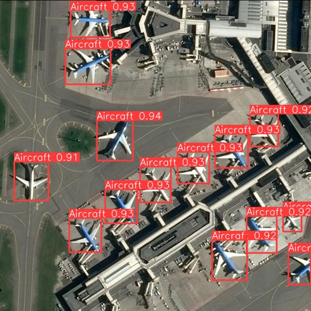
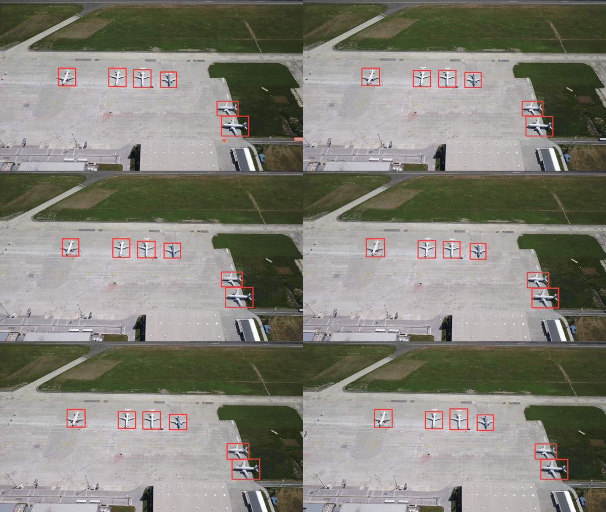
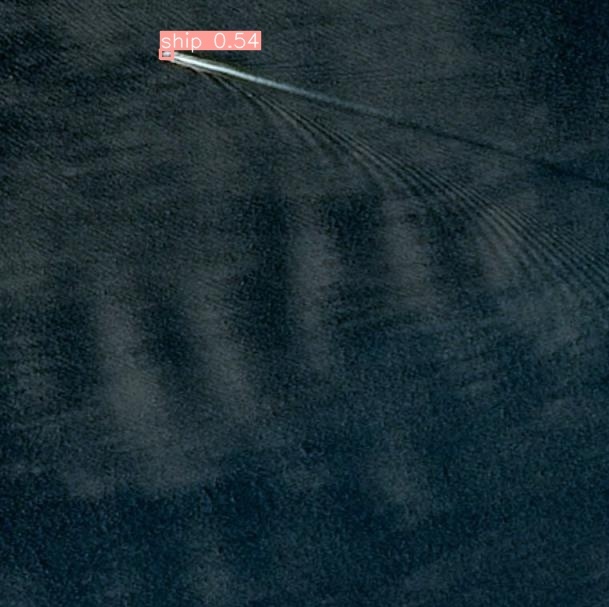
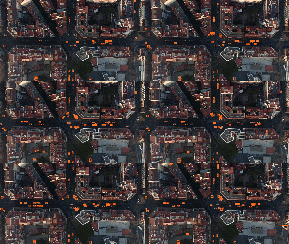
Metrics like mAP50 can only be interpretable to some extent. The real question here is how do these models perform in the real-world? Let’s now look at some image and video inference using the best weights from the fine-tuning YOLOv9 experiments that were conducted earlier in this research work.

Aerial Airplane Detection

Image Inference: 640×640

Video Inference: 567×1024

Aerial Ship Detection

Image Inference: 640×640

Video Inference: 567×1024

Aerial Vehicle Detection

Image Inference: 640×640

Video Inference: 567×1024

NOTE: All of the inference footage used in this section was taken from the licensed Envato Elements stock video library.

GELAN v/s SPPF Feature Map Activation Visualization

Highlights

• GELAN’s feature maps showcase a consistent and efficient distribution of features due to its gradient propagation-focused design, ensuring uniform quality across all network depths.
• SPPF emphasizes multi-scale feature representation, enabling YOLOv8 to adeptly capture and detect objects of varying sizes and shapes through its spatially diverse pooling strategy.
• While GELAN prioritizes depth-efficient and stable feature extraction, SPPF strengthens the model’s adaptability to different object dimensions, highlighting a contrast in architectural focus.

GELAN (Generalized Efficient Layer Aggregation Network) in YOLOv9 is designed to focus on gradient path optimization and computational efficiency. It utilizes computational blocks like CSP (Cross Stage Partial) networks to streamline the gradient flow and minimize redundancy in parameters and computations.

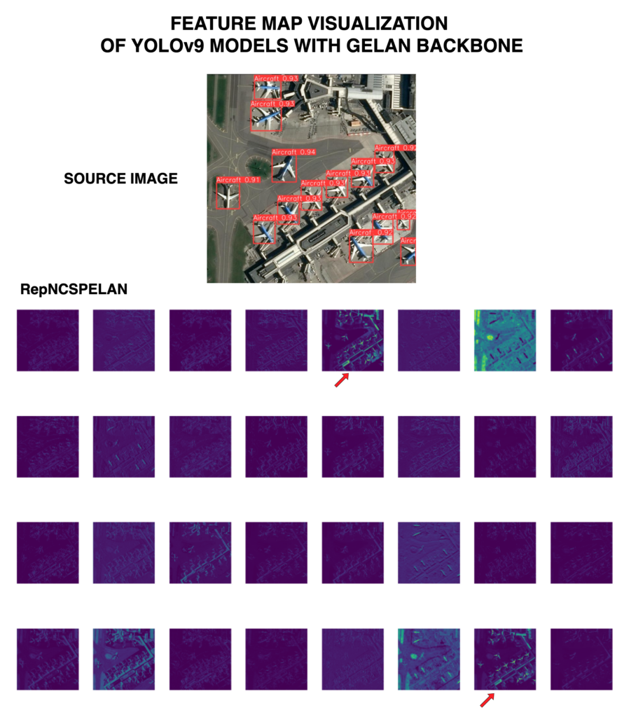
From FIGURE 16, it can be inferred that the quality of feature extraction in the feature maps indicated using red arrows is phenomenal! Through ablation studies, GELAN has demonstrated its robustness in maintaining performance across various block types, with CSP blocks showing particular efficacy in enhancing average precision. This architecture’s resilience to depth variations indicates its stable feature extraction capability across different network layers, which is crucial for consistent object detection performance irrespective of the object’s scale.

In contrast, SPPF in YOLOv8 functions as a multi-scale feature aggregator that pools features at various scales to create a comprehensive representation of the input image. By integrating SPPF, the model achieves a versatile detection capability, efficiently recognizing objects of varying sizes through a singular consolidated feature map. This fusion process significantly reduces FLOPs, enhancing the model’s computational efficiency without compromising the richness of the multi-scale feature representation.

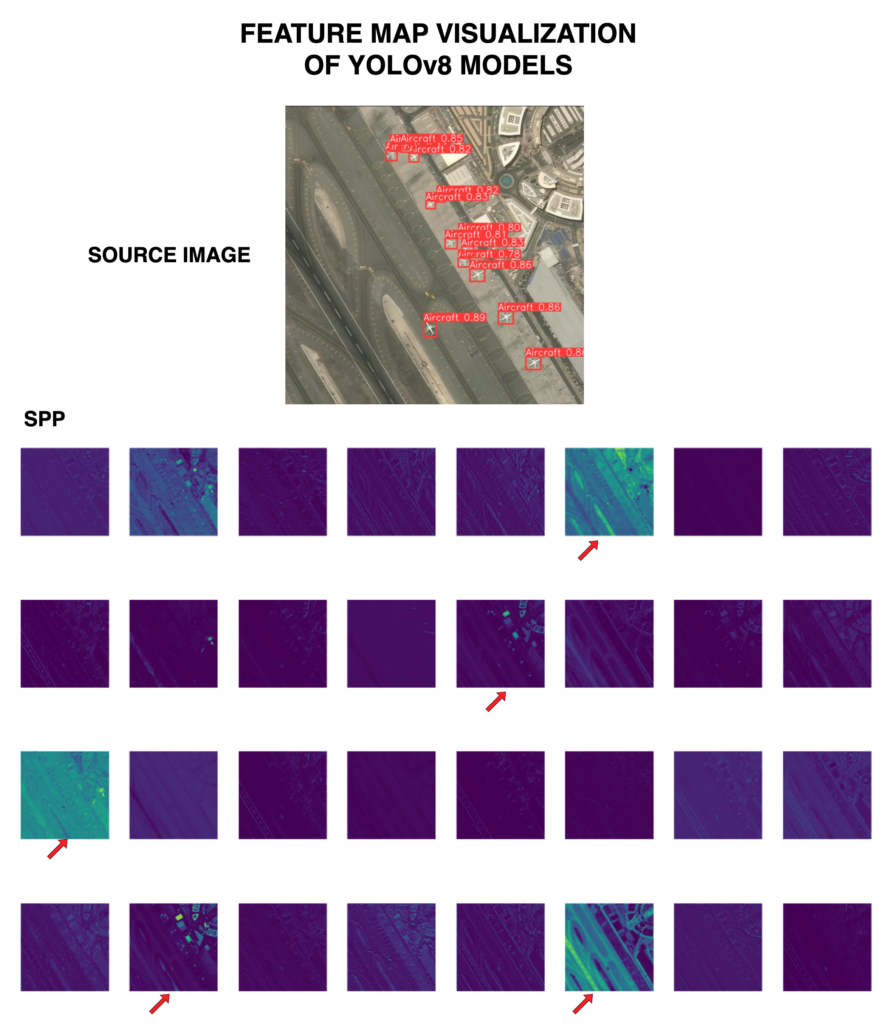
From FIGURE 17, it can be observed that compared to GELAN, the quality of feature extraction of the airplanes is not clear. Now, this makes a drastic difference! 

When visualizing feature maps from both architectures, GELAN’s output would likely exhibit a more uniform distribution of informative features across layers, reflecting its design goal of efficient gradient propagation and consistent feature quality at all depths. This could result in a more stable and predictable feature set for object detection, with less variance in feature quality as the network depth increases.

On the other hand, feature maps from SPPF would display a diverse range of spatial resolutions, capturing a broad spectrum of object sizes and shapes. This diversity is a direct consequence of SPPF’s multi-scale pooling, which amalgamates features across various spatial dimensions, ensuring that the model’s detection capabilities remain robust across different object scales.

Interesting results, right? SCROLL UP or have a look at the code walkthrough section to explore the intricate fine-tuning procedure.

Key Takeaways

The following points summarize the key research findings on improving YOLOv9 models for better object detection performance and efficiency.

• Fine-tuning YOLOv9 on the SkyFusion dataset significantly improved object detection, achieving an mAP50 of 0.713 through strategic modifications like learning rate adjustments and backbone freezing.
• GELAN, with its emphasis on efficient gradient flow, demonstrated superior performance and stability across various computational blocks, especially CSP blocks which enhanced average precision by 0.7%.
• Aerial object detection in images and videos showcased the practical efficacy of the fine-tuned YOLOv9 models, highlighting their robustness in real-world applications.
• Comparative feature map visualization revealed GELAN’s consistent and uniform feature distribution, while SPPF in YOLOv8 underscored the model’s multi-scale feature aggregation capability, catering to objects of diverse sizes.

Conclusion

This article throws light on the significant impact of fine-tuning YOLOv9 models on custom datasets, notably enhancing detection accuracy as evidenced by the SkyFusion dataset results. 

The introduction of the GELAN architecture within YOLOv9 has proven to be a substantial advancement, optimizing both gradient flow and computational efficiency. Through meticulous experimentation and analysis, this study not only advances the field of object detection but also sets a new benchmark for future explorations in optimizing deep learning models for specific datasets.

References

[1] Wang, Chien-Yao, Hong-Yuan Mark Liao, and I-Hau Yeh. “Designing network design strategies through gradient path analysis.” arXiv preprint arXiv:2211.04800 (2022).

[2] Wang, Chien-Yao, I-Hau Yeh, and Hong-Yuan Mark Liao. “YOLOv9: Learning What You Want to Learn Using Programmable Gradient Information.” arXiv preprint arXiv:2402.13616 (2024).

Click here to download the source code to this post