FCOS- Anchor Free Object Detection Explained

FCOS: Fully Convolutional One-stage Object Detection is an anchor-free (anchorless) object detector. It solves object detection problems in a per-pixel prediction fashion, similar to segmentation. Most of the recent anchor-free or anchorless deep learning-based object detectors use FCOS as a basis. 

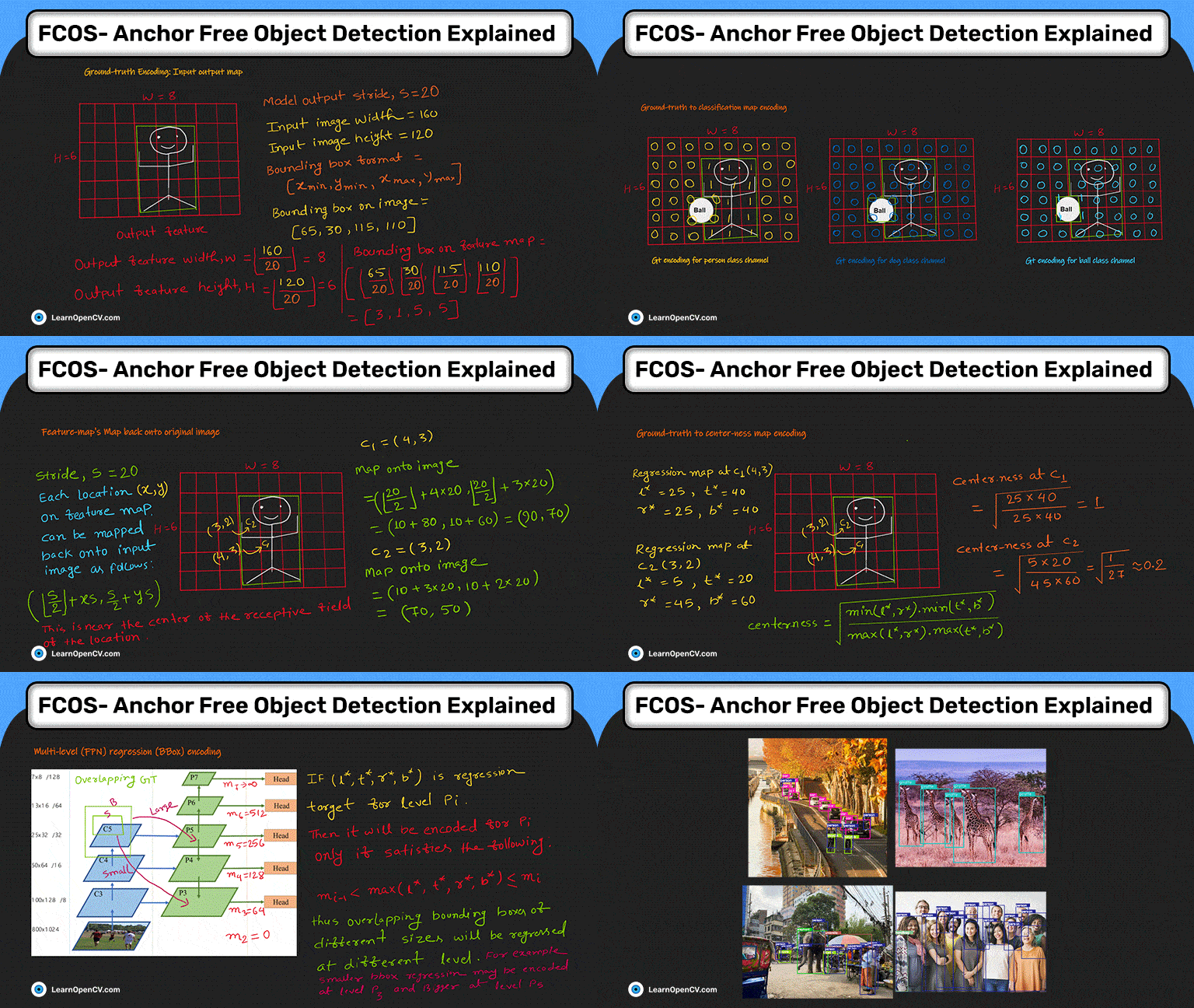
In this article, we will discuss the following:

1. Fundamentals of FCOS: The model architecture, ground truth encoding, prediction decoding, and loss function.
2. The intuitive explanation of all fundamental concepts. 
3. Where FCOS stands compared to other object detection models.
4. We will also present FCOS inference using PyTorch and TorchVision on images and videos.

People who can make the best use of the article: 

1. Those who want to understand the deep learning classification pipeline and want intuitively learn deep learning-based object detection.
2. Have experience in anchor-based object detection and want to explore anchor-free object detection.
3. Want to take a deeper look into FCOS – Fully Convolutional One-stage Object Detection
4. Wanted to create an application using a pre-trained object detection model.

• Fundamentals of Object Detection
• Architecture of The FCOS Model
• Ground Truth Encoding in FCOS
• Model Prediction Decoding in FCOS
• Loss Functions in FCOS
• How does FCOS work?
• FCOS Results
• FCOS Model Inference using PyTorch
• Recommended Readings
• Summary

Fundamentals of Object Detection

Deep learning-based object detection is broadly divided into two types:

• Anchor-based object detection, and
• Anchor-free (anchorless) object detection

Centernet – Objects as points explain the fundamentals of deep learning-based object detection. If you are not familiar with the fundamentals of object detection, read the following sections:

1. What is Object Detection in Machine Learning/Deep Learning? 
2. What is an Anchor in Object Detection?
3. What is Anchor-Based Object Detection?
4. What is Anchor-Free Object Detection?
5. Is Anchor-Free Better Than Anchor-based Object Detection?
6. Components of Deep Learning-Based Object Detection.

An object detection model has the following components in the pipeline:

1. Object detection model,
2. Ground truth encoding,
3. Loss function, and
4. Model prediction decoding

Assuming you understand these components, we will explain FCOS: Fully Convolutional One-Stage Object Detection in this framework.

Architecture of The FCOS Model

FCOS stands for Fully Convolutional One-stage Object Detection. It is motivated by FCN: Fully Convolutional Networks for semantic segmentation. It uses similar pixel-wise prediction for object detection. Let us see how it does it. 

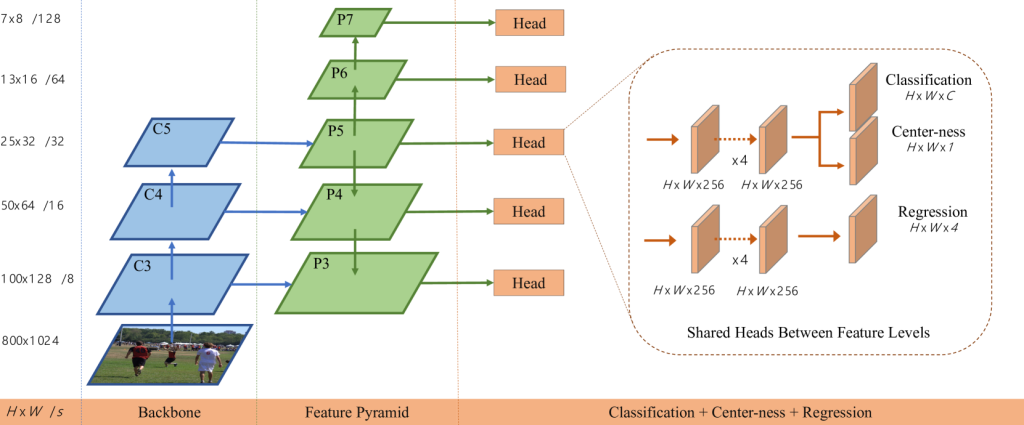
The above figure (fig. 1) depicts the network architecture of FCOS. It has three parts:

1. Backbone,
2. Feature Pyramid, and
3. Head

Three feature maps from the backbone, C3, C4, and C5, feed into the feature pyramid network (FPN) at P3, P4, and P5, respectively. Furthermore, the output of P5 is fed into P6, and the output of P6 is fed into P7.

The output of P3 to P7 goes into a head network.

If we zoom into the head network, it can be seen to have two branches:

1. For classification: It has two parts, one for class confidence prediction and the other to predict the center-ness of the object. You already learned what class confidence is in the object detection context. We will go over center-ness in detail later in the article. 
2. For regression: The regression branch is responsible for predicting the bounding.

The feature output shape shown in the image is for an input image size of 800 x 1024. 

The output strides (downsampling ratio to the input image size) at C3/P3, C4/P4, C5/P5, P6, and P7 are 8, 16, 32, 64, and 128, respectively. As it goes up, output resolution decreases; for example, output width and height at level C3/P3 is 100 x 128, and level C4/P4 is 50 x 64. 

The head output width and height depend on their level. For example, the width and height at level P7 are 7 x 8, and at level P6, they are 13 x 16, respectively. However, at all levels, depth is the same and is as follows:

1. Classification depth is C, where C is the number of object classes.
2. Center-ness depth is one. Hence, it predicts the center-ness quality of the bounding; one scalar is sufficient to represent quality. 
3. The regression depth is four because four numbers are required to represent a bounding box in a 2-D plane.

Ground Truth Encoding in FCOS

Understanding ground truth encoding is essential as recent anchorless object detectors use similar encoding, for example, the YOLOx object detector and YOLOv6 object detection. 

Let us now delve deeper into FCOS encoding. 

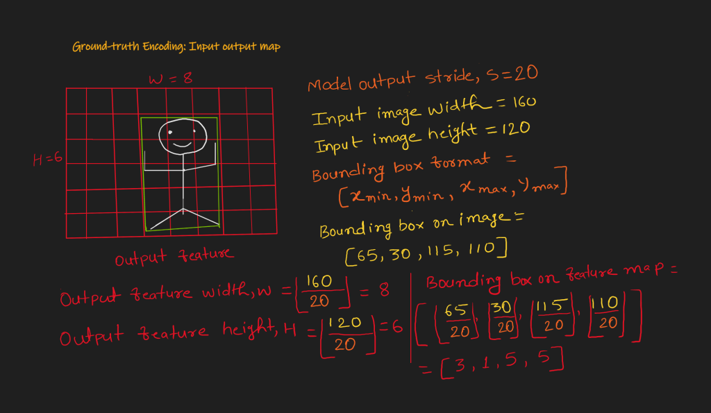
For an illustration of encoding, let us assume the model has only one level output and the model stride, s is 20.

The input image is 160 x120, so the output feature will be 8 x 6, as shown below (fig. 2).

The bounding box format is .

The bounding box on the feature map (explanation in fig. 2):

Each output feature needs a corresponding label. The label should come from the ground truth. This means we need to encode the ground truth so that its structure matches the output features structure.

Hence the ground truth needs to map with three model outputs:

1. Classification
2. Center-ness, and
3. Regression

Ground-truth to Classification Map Encoding

Let’s consider three classes (person, dog, and ball) without including the background class. In this case, the FCOS classification map will have three channel outputs, one for each class.

Labeling a channel only depends on bounding boxes belonging to the class for which the channel is responsible. For example, look at the image below (fig. 3).

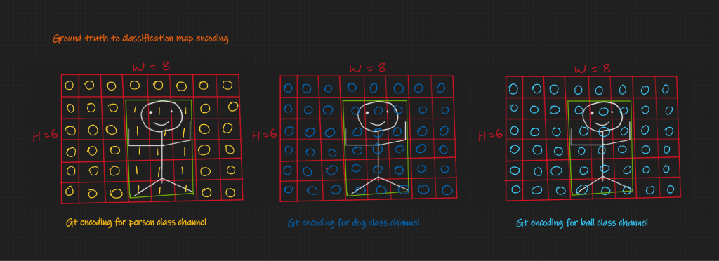
For the person class channel, values inside the bounding box are one, and the other values are zero. All values for the other class channels are zero because there is no instance for dog and ball.

What if Two Bounding Boxes Overlap?

If two bounding boxes overlap, the label of the smaller bounding box will be the label for classification. So bounding box is also regressed for the label, which has a smaller bounding box. For example, look at the image below (fig. 4).

The smaller bounding box has fewer representations in the classification map. So it makes sense to prioritize it. 

How is it Taking Care of the Background (no object class)?

For a given and coordinate, if all values across the depth (channels) are zero, then the cell is a background label. In other words, if a cell does not have the value of 1 for any channel, the cell belongs to the background.

How does location on the feature map back onto the input image?

Look at the image below (fig. 5). Here, mapping for two points, and , is shown.

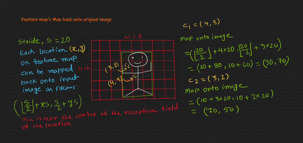
Note that the mapped point in the original image is near the center of the receptive field location.

Before discussing the FCOS center-ness map encoding, let’s talk about regression map encoding.

Ground-truth to Regression Map Encoding

The model predicts the bounding box for the point where the class label is one.

It has four channels to predict four numbers for the bounding box.

The regression map encoding has the following four numbers:

1. distance of the left edge, ,
2. distance of the top edge, ,
3. distance of the right edge, , and
4. distance of the bottom edge,  

The image below (fig. 6) demonstrates the FCOS regression map encoding calculation.

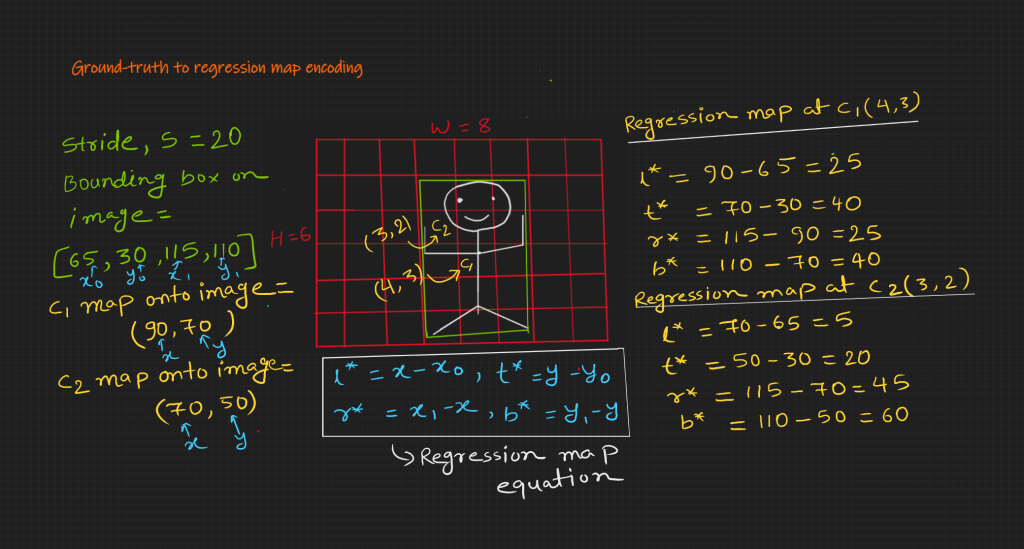
We know that in the case of bounding box overlap, we will choose the smallest bounding box for regression. However, in the case of multi-level outputs, overlapping on the same feature map will be rare. 

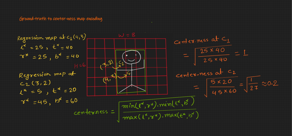
Ground-truth to Center-ness Map Encoding

There is one channel for center-ness. As the name suggests, if a point is at the center of the bounding box, its value should be one, and as the point goes away from the center, its value should decrease.

The below image (fig. 7) has the equation for center-ness and demonstrates the calculation of center-ness map encoding.

Here is an example of an FCOS center-ness heatmap of an image below (fig. 8).

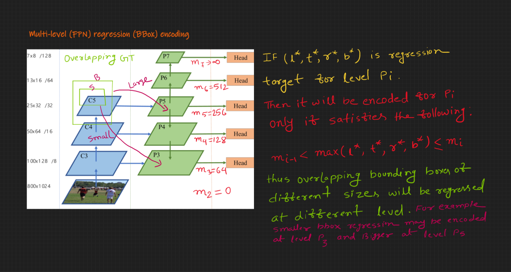
Ground truth Encoding for Multi-Level (FPN) Prediction in FCOS

Encoding steps remain the same for multi-levels. However, different level outputs have different strides. Hence encoding strides for the corresponding level should be used. 

All bounding boxes need not be encoded at all levels. Roughly, smaller bounding boxes will be encoded at larger feature maps and vice versa.

The below image (fig. 9) demonstrates the bounding box and feature level mapping criteria. 

What is the Benefit of Multi-Level (FPN) in FCOS?

1. Initial features (starting from input) have more localization and less object information. However, later layers have more objectness and less localization information. For example, in the above image (fig. 9), C3 is the initial feature, and C5 is the later feature. Here in Feature Pyramid, P5 goes into P4 and P4 into P3. Here, the connection provides more object information to the initial layers. 
2. Another major benefit is high BPR (best possible recall). 

What is BPR (best possible recall) in Object Detection?

The Upper bound of the recall rate that a detector can achieve is called BPR (Best Possible Recall). It is not a model prediction recall; instead, it’s a ground truth encoding recall.

Generally, recall is used in the context of prediction. So what is a recall in encoding?

When we encode the ground truth, it is possible that a few ground truths may have encoded representation in the training sample due to encoding algorithm limitations.

This makes it clear what BPR is and why it is important.

How does FPN (multi-level output) in FCOS help in high BPR?

Suppose there are two bounding boxes. One is slightly smaller and is entirely inside, the bigger one. 

For a single output, for a given stride, both boxes may have the same classification map. In this case, for the given algorithm, smaller bounding will have encoded maps but bigger will not. Hence there is no mapping for the bigger bounding box.

However, in the case of multi-level outputs, there may be other layers that can accommodate the bigger bounding box.

Below is a table from the paper that compares the BPR of RetinaNet and FCOS.

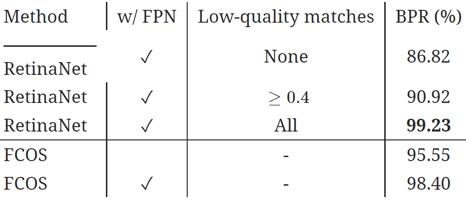
Here, you can see that even with FPN, BPR is not 100%.

Model Prediction Decoding in FCOS

Prediction decoding means converting model prediction to standard ground truth format.

The model inference decoding steps are as follows:

1. From the classification head output, get the confident location. For example, locations with a score of more than 0.5 may be considered confident locations if there are three object classes. 
2. For confident locations, get regression output from the regression head. 
3. Calculate the width (l + r) and height (t + b) from the regression output. 
4. Map confident locations back to the input image.
5. Get the center-ness value for confident locations from the center-ness head.
6. Update the confidence score by multiplying it by the center-ness value.

Next, use NMS to filter decoded bounding boxes.

100K+ Learners
3 Hours of Learning

Join Free OpenCV Bootcamp

15K+ Learners
3 Hours of Learning

Join Free TensorFlow Bootcamp

10K+ Learners
8 Hours of Learning

Join Free PyTorch Bootcamp

View all AI Free Courses

Loss Functions in FCOS

There are three loss functions for the output head (fig. 10):

1. Classification loss: It uses focal loss.
2. Regression loss: It is IoU loss.
3. Center-ness loss: It is BCE (binary cross-entropy error) loss.

It is important to note that multiple positive samples exist for single bounding boxes. So it makes the positive vs. negative sample less skewed. It makes the training stable.

Now that we have learned the fundamentals of FCOS, now let’s summarize it in the following section.

How does FCOS work?

• FCOS uses Resnet-FPN architecture. So it outputs different resolutions. The FPN architecture helps in high BPR (Best Possible Recall) and better prediction recall.
• For training the model, ground truths bounding boxes need to be encoded in a particular way; this is also the nobility of FCOS. This unique way helps the model to have a less skewed training sample.
• It uses three loss functions – a focal loss for classification, BCE loss for center-ness, and IoU loss for regression.
• It requires decoding of model prediction for getting standard ground truth format. 

FCOS Results

Here is a table that compares the mAP of RetinaNet and FCOS.

You can see FCOS outperforms RetinaNet.
The following table compares the mAP of FCOS with other state-of-the-art object detection models.

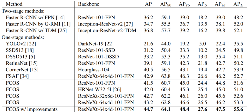
You can see FCOS outperforms other state-of-the-art models.

Click here to download the source code to this post

FCOS Model Inference using PyTorch

FCOS model is available in torchvision. Let us use the pre-trained model for image and video inference.

import torch
import numpy as np
import cv2
import torchvision
import torchvision.transforms as transforms
import matplotlib.pyplot as plt
import glob
import os
import time
import requests 
import zipfile

Utils

Let us write different utils functions that are needed for inference and visualization.

Create a directory to save inference results.

# Create result directory.
result_dir = 'results'
os.makedirs(result_dir, exist_ok=True)

Let’s use GPU (Cuda) if available.

device = torch.device('cuda' if torch.cuda.is_available() else 'cpu')
print('Using {}.'.format(device))

Using cuda.

The pre-trained model is trained on the COCO dataset. The model predicts the class index. To map it to the class name, let us define the COCO class name list.

COCO_CLASSES = [
    '__background__', 'person', 'bicycle', 'car', 'motorcycle', 'airplane', 'bus',
    'train', 'truck', 'boat', 'traffic light', 'fire hydrant', 'N/A', 'stop sign',
    'parking meter', 'bench', 'bird', 'cat', 'dog', 'horse', 'sheep', 'cow',
    'elephant', 'bear', 'zebra', 'giraffe', 'N/A', 'backpack', 'umbrella', 'N/A', 'N/A',
    'handbag', 'tie', 'suitcase', 'frisbee', 'skis', 'snowboard', 'sports ball',
    'kite', 'baseball bat', 'baseball glove', 'skateboard', 'surfboard', 'tennis racket',
    'bottle', 'N/A', 'wine glass', 'cup', 'fork', 'knife', 'spoon', 'bowl',
    'banana', 'apple', 'sandwich', 'orange', 'broccoli', 'carrot', 'hot dog', 'pizza',
    'donut', 'cake', 'chair', 'couch', 'potted plant', 'bed', 'N/A', 'dining table',
    'N/A', 'N/A', 'toilet', 'N/A', 'tv', 'laptop', 'mouse', 'remote', 'keyboard', 'cell phone',
    'microwave', 'oven', 'toaster', 'sink', 'refrigerator', 'N/A', 'book',
    'clock', 'vase', 'scissors', 'teddy bear', 'hair drier', 'toothbrush'
]

After model inference, we need to plot the predicted bounding box. It is suggested to use different colors for different classes.

# Create different colors for each class.
np.random.seed(42)
COLORS = np.random.uniform(0, 255, size=(len(COCO_CLASSES), 3))

Here is a function that downloads FCOS (fcos_resnet50_fpn) model weight using torchvision, loads it, and returns it in eval mood.

# Function to load the model.
def get_model(device):
    # Load the model.
    model = torchvision.models.detection.fcos_resnet50_fpn(
        weights='DEFAULT'
    )
    # Load the model onto the computation device.
    model = model.eval().to(device)
    return model

Before inference, the input images need to have some standard transformation. We use the most basic to transform to tensor.

# Define the torchvision image transforms.
transform = transforms.Compose([
    transforms.ToTensor()
])

Here is a function to visualize four images in a 2 x 2 grid.

# Plot and visualize images in a 2x2 grid.
def visualize(result_dir):
    """
    Function accepts a list of images and plots
    them in a 2x2 grid.
    """
    plt.figure(figsize=(20, 18))
    image_names = glob.glob(os.path.join(result_dir, '*.jpg'))
    for i, image_name in enumerate(image_names):
        image = plt.imread(image_name)
        plt.subplot(2, 2, i+1)
        plt.imshow(image)
        plt.axis('off')
    plt.tight_layout()
    plt.show()

Download Data

The following functions are for downloading and unzipping data.

def download_file(url, save_name):
    url = url
    if not os.path.exists(save_name):
        file = requests.get(url)
        open(save_name, 'wb').write(file.content)
        
download_file(
    'https://www.dropbox.com/s/ukc7wocsn7xrm2r/data.zip?dl=1',
    'data.zip'
)

# Unzip the data file
def unzip(zip_file=None):
    try:
        with zipfile.ZipFile(zip_file) as z:
            z.extractall("./")
            print("Extracted all")
    except:
        print("Invalid file")

unzip('data.zip')

Extracted all

Prediction Function

Let us write a function for inference. It takes images, the model, which device to use (GPU or CPU), and the bounding box threshold. And it returns bounding boxes coordinates, class names, and the class index.

def predict(image, model, device, detection_threshold):
    """
    Predict the output of an image after forward pass through
    the model and return the bounding boxes, class names, and 
    class labels. 
    """
    # Transform the image to tensor.
    image = transform(image).to(device)
    # Add a batch dimension.
    image = image.unsqueeze(0) 
    # Get the predictions on the image.
    with torch.no_grad():
        outputs = model(image) 

    # Get score for all the predicted objects.
    pred_scores = outputs[0]['scores'].detach().cpu().numpy()

    # Get all the predicted bounding boxes.
    pred_bboxes = outputs[0]['boxes'].detach().cpu().numpy()
    # Get boxes above the threshold score.
    boxes = pred_bboxes[pred_scores >= detection_threshold].astype(np.int32)
    labels = outputs[0]['labels'][pred_scores >= detection_threshold]
    # Get all the predicited class names.
    pred_classes = [COCO_CLASSES[i] for i in labels.cpu().numpy()]

    return boxes, pred_classes, labels

Annotation Functions

Here is a function that takes bounding boxes, their class name, class index, and the inferred image and returns annotated image.

def draw_boxes(boxes, classes, labels, image):
    """
    Draws the bounding box around a detected object.
    """
    lw = max(round(sum(image.shape) / 2 * 0.003), 2) # Line width.
    tf = max(lw - 1, 1) # Font thickness.
    
    for i, box in enumerate(boxes):
        p1, p2 = (int(box[0]), int(box[1])), (int(box[2]), int(box[3]))
        color = COLORS[labels[i]]
        class_name = classes[i]
        cv2.rectangle(
            image,
            p1,
            p2,
            color[::-1],
            thickness=lw,
            lineType=cv2.LINE_AA
        )
        # For filled rectangle.
        w, h = cv2.getTextSize(
            class_name, 
            0, 
            fontScale=lw / 3, 
            thickness=tf
        )[0]  # Text width, height
        
        outside = p1[1] - h >= 3
        p2 = p1[0] + w, p1[1] - h - 3 if outside else p1[1] + h + 3
        
        cv2.rectangle(
            image, 
            p1, 
            p2, 
            color=color[::-1], 
            thickness=-1, 
            lineType=cv2.LINE_AA
        )  
        cv2.putText(
            image, 
            class_name, 
            (p1[0], p1[1] - 5 if outside else p1[1] + h + 2),
            cv2.FONT_HERSHEY_SIMPLEX, 
            fontScale=lw / 3.8, 
            color=(255, 255, 255), 
            thickness=tf, 
            lineType=cv2.LINE_AA
        )
    return image

Inference on Images

Now that we have the required utils, 

let’s make inferences.

Get the model.

model = get_model(device)

Downloading: "https://download.pytorch.org/models/fcos_resnet50_fpn_coco-99b0c9b7.pth" to /root/.cache/torch/hub/checkpoints/fcos_resnet50_fpn_coco-99b0c9b7.pth
100%
124M/124M [00:08<00:00, 19.0MB/s]

Make inferences and plot bounding boxes and their class name on the image.

# Get all the image paths.
image_paths = glob.glob(os.path.join('data', '*.jpg'))

# Run inference on all images.
for image_path in image_paths:
    # Read the image.
    image = cv2.imread(image_path)
    # Create a BGR copy of the image for annotation.
    image_bgr = cv2.cvtColor(np.array(image), cv2.COLOR_RGB2BGR)
    # Detect outputs.
    boxes, classes, labels = predict(
        image, 
        model, 
        device, 
        detection_threshold=0.5
    )
    # Draw bounding boxes.
    image = draw_boxes(boxes, classes, labels, image_bgr)
    save_name = image_path.split(os.path.sep)[-1]
    cv2.imwrite(os.path.join(result_dir, save_name), image[:, :, ::-1])

Finally, visualize the results.

# Visualize
visualize(result_dir)

Inference on Videos

Let’s make inferences from the model on videos.

It will load the video, make inferences on each frame, add detection, and save it back to the video.

# Get all the video paths.
video_paths = glob.glob(os.path.join('data', '*.mp4'))

for video_path in video_paths:
    print(f"Running inference on video: {video_path}")
    cap = cv2.VideoCapture(video_path)

    if (cap.isOpened() == False):
        print('Error while trying to read video. Please check path again')

    # Get the frame width and height.
    frame_width = int(cap.get(3))
    frame_height = int(cap.get(4))

    save_name = video_path.split(os.path.sep)[-1]
    # Define codec and create VideoWriter object .
    out = cv2.VideoWriter(os.path.join(result_dir, save_name), 
                          cv2.VideoWriter_fourcc(*'mp4v'), 
                          30, 
                          (frame_width, frame_height))

    frame_count = 0 # To count total frames.
    total_fps = 0 # To get the final frames per second.
    
    # Read until end of video.
    while(cap.isOpened):
        # Capture each frame of the video.
        ret, frame = cap.read()
        if ret:
            frame_copy = frame.copy()
            frame_copy = cv2.cvtColor(frame_copy, cv2.COLOR_BGR2RGB)
            # Get the start time.
            start_time = time.time()
            # Get predictions for the current frame.
            boxes, classes, labels = predict(
                frame, 
                model, 
                device, 
                detection_threshold=0.5
            )

            # Draw boxes and show current frame on screen.
            image = draw_boxes(boxes, classes, labels, frame)

            # Get the end time.
            end_time = time.time()
            # Get the fps.
            fps = 1 / (end_time - start_time)
            # Add fps to total fps.
            total_fps += fps
            # Increment frame count.
            frame_count += 1
            if frame_count % 100 == 0:
                print(f"Frame: {frame_count}   ::   FPS: {fps:.1f}")
            # Write the FPS on the current frame.
            cv2.putText(image, f"{fps:.3f} FPS", (15, 30), cv2.FONT_HERSHEY_SIMPLEX,
                        1, (0, 255, 0), 2)
            # Convert from BGR to RGB color format.
#             cv2.imshow('image', image)
            out.write(image)
            # Press `q` to exit.
#             if cv2.waitKey(1) & 0xFF == ord('q'):
#                 break

        else:
            break

    # Release VideoCapture().
    cap.release()
    # Close all frames and video windows.
    cv2.destroyAllWindows()

    # Calculate and print the average FPS.
    avg_fps = total_fps / frame_count
    print(f"Average FPS: {avg_fps:.3f}\n\n")

Running inference on video: data/soccer.mp4
Frame: 100   ::   FPS: 8.8
Frame: 200   ::   FPS: 8.4
Frame: 300   ::   FPS: 8.8
Average FPS: 8.929


Running inference on video: data/horses_video.mp4
Frame: 100   ::   FPS: 8.8
Frame: 200   ::   FPS: 9.3
Average FPS: 8.748


Running inference on video: data/traffic_video.mp4
Frame: 100   ::   FPS: 7.6
Frame: 200   ::   FPS: 7.3
Frame: 300   ::   FPS: 7.3
Frame: 400   ::   FPS: 7.2
Frame: 500   ::   FPS: 7.4
Frame: 600   ::   FPS: 7.4
Frame: 700   ::   FPS: 7.4
Frame: 800   ::   FPS: 7.5
Frame: 900   ::   FPS: 7.5
Frame: 1000   ::   FPS: 7.3
Frame: 1100   ::   FPS: 7.3
Frame: 1200   ::   FPS: 7.4
Average FPS: 7.433


Running inference on video: data/cowboy.mp4
Frame: 100   ::   FPS: 7.3
Frame: 200   ::   FPS: 7.3
Frame: 300   ::   FPS: 7.5
Frame: 400   ::   FPS: 7.2
Frame: 500   ::   FPS: 7.3
Frame: 600   ::   FPS: 7.4
Frame: 700   ::   FPS: 7.5
Average FPS: 7.393

Sample Videos Outputs

Recommended Readings

Here are a few similar blog posts that you may be interested in.

• YOLOv7 Object Detection Paper Explanation and Inference
• Fine Tuning YOLOv7 on Custom Dataset
• YOLOv7 Pose vs. MediaPipe in Human Pose Estimation
• YOLOv6 Object Detection – Paper Explanation and Inference
• YOLOX Object Detector Paper Explanation and Custom Training
• Object Detection using YOLOv5 and OpenCV DNN in C++ and Python
• Custom Object Detection Training using YOLOv5
• Pothole Detection using YOLOv4 and Darknet

Summary

Let us summarize all the points that we have studied about FCOS so far

1. The FCOS is motivated by FCN – Fully Convolutional Networks.
2. It uses FPN-based architecture that helps in high BPR, Best  Possible Recall, and better prediction recall.
3. We have also seen how the ground truth is encoded and model predictions decoded in FCOS. Its encoding method helps get more object (positive) samples during training, which leads to stable training.
4. FCOS uses three loss functions: focal loss, BCE loss, and IoU loss.
5. We have seen how its performance compares to the other models.
6. We have also seen how pre-trained models can be used for image and video inference.

References

1. FCOS: Fully Convolutional One-Stage Object Detection
2. Feature Pyramid Networks for Object Detection
3. Torchvision FCOS