Distributed Parallel Training: PyTorch Multi-GPU Setup in Kaggle T4x2

Training modern deep learning models often demands huge compute resources and time. As datasets grow larger and model architecture scale up, training on a single GPU is inefficient and time consuming. Modern vision models or LLM doesn’t fit into a memory constraints of a single GPU. Attempting to do so often leads to:

• CUDA Out of Memory (OOM) errors
• Reliance on model quantization, layer pruning or distillation, often at the expense of precision.
• Use of gradient checkpointing, which trades memory for compute, to simulate large batch training.

These workarounds may lead to suboptimal model performance or increase in training complexity. This is where distributed training comes to rescue. It is the process of training models across multiple devices and makes not only feasible to train large models but also drastically speeding up the overall training time. PyTorch has an excellent support for production ready distributed training.

This articles aims to a one-stop reference guide for understanding the different types of distributed training in PyTorch. Having prior knowledge of Autograd and model training is assumed. As a hands-on experience, we will walk through scripts to setup a Single Node Multi-GPU training using Kaggle T4x2 GPU runtime.

Let the GPUs Go Brrr. 🏎️💨.

GPU Memory Consumption

Before discussing about distributed training, it’s important to understand about different operations and process that consume GPU memory during training.

Total Memory =
Model Memory + Optimizer State +
max⁡(Gradients,Optimizer Intermediates, Activations)

• Model Parameters: The weights and biases of the neural network
• Gradients: Stored for each trainable parameter during the backward pass, same sizes as model parameters
• Activations: Intermediate outputs of layers saved during the forward pass, needed for gradient computation in the backward pass. Their size depends on batch size and model architecture.
• Optimizer States: Additional variables maintained by optimizers (eg. momentum, adaptive learning rate). For instance the Adam optimizer typically consumes 2x the model parameter size in memory.
• Optimizer Intermediates: Some optimizers might have temporary buffers during the step() call.

The cumulative memory footprint of these components can easily exceed the capacity of a single GPU, particularly LLMs, VLMs etc. This necessitates distributing the model and data across multiple devices or even nodes for efficient training. Here, a node typically refers to a single physical computer or server which may itself contain one or more GPUs.

• Single-Node, Multi-GPU: Training leverages multiple GPUs housed within one such physical machine (node). This is a common setup for accelerating training when model and data sizes are moderately large.
• Multi-Node, Multi-GPU: For even greater scale, training utilizes GPUs spread across several interconnected physical machines (nodes). This approach is essential for the largest models and dataset, requiring a network to connect these nodes.

👉 Did you know that models like LLAMA-4 or Grok-3 are trained on clusters with nearly 100k H100 GPUs, running distributed workloads across multiple nodes for several days.

100K+ Learners
3 Hours of Learning

Join Free OpenCV Bootcamp

15K+ Learners
3 Hours of Learning

Join Free TensorFlow Bootcamp

10K+ Learners
8 Hours of Learning

Join Free PyTorch Bootcamp

View all AI Free Courses

Common Terminologies in Distributed Computing

• Process Group (dist.ProcessGroup):
  • A collection of processes that participate in a distributed job. All communication happens within a process group.
  • PyTorch creates a default ‘world’ process group when initialized, composed of all participant processes.

• World Size:
  • The total number of processes participating in the distributed training job. We will use single process per GPU for simplicity.
  • Let’s say we have 2 machines (nodes) and each machine uses 4 GPUs, with one process per GPU, the world size is 8,

world_size = num_nodes * num_gpus_per_node

• Global Rank:
  • A unique integer ID assigned to each process (device) within the process group ranging from 0 to world_size - 1. This is the global rank across all nodes and processes.

• Local Rank
  • A unique integer ID assigned to each process within a single machine ( per node).
  • For eg, if a node has 4 GPUs, the processes on that node will have local_rank from 0 and 3.

• Master Node / Process (Rank 0)
  • Master node is the central controller that orchestrates and coordinates all activities within the compute cluster in an efficient manner. By convention, the process with rank=0 is often designated as the “master” or “main” process. It’s responsible for tasks like scheduling jobs, resource management and distributing work across all the worker nodes.

Communication Backends

For these distributed processes to colloborate, they need a way to talk to each other. PyTorch’s torch.distributed package manages this through communication backends and initialization methods using torch.distributed.init_process_group()

The backend parameter in init_process_group() specifies the library that we will use to exchange data between process.

• NCCL (Nvidia Collective Communication Library)
  • The Gold Standard for Nvidia GPUs. NCCL is highly optimized for inter-GPU communication, both within a single node (leveraging NVLink) and across multiple nodes. It provides efficient implementation of collective operations like all_reduce, broadcast, gather etc.
    

• Gloo (FAIR Meta)
  • A platform agnostic backend that works for both CPU and GPU-based communication.
  • For GPUs, it typically involves copying data from GPU to CPU memory, performing network communication (eg. via TCP/IP), and then copying back to GPU. This makes it slower than NCCL for GPU tasks. This backend is used as a fallback if NCCL setup is problematic or specific operations are not optimized in NCCL.

• MPI (Message Passing Interface)
  • A widely adopted standard and portable API in High-Performance Computing (HPC) to build scalable applications on multi-node compute clusters by communicating data via messages between distributed processes.
  • MPI provides functions for point-to-point communication (like sending and receiving messages) and collective communication (such as broadcasting, scattering and gathering data across processes).

Initialization Methods

Once the backend is chosen, processes need a way to find each other and agree on roles (who is rank 0, rank 1 etc.). This is a synchronization step specificed by init method.

• Environment Variable Initialization (init_method="env://"):
  • Processes read connection details from environment variables.
    • MASTER_ADDR: IP address or hostname of the master node (hosting rank 0)
    • MASTER_PORT: A free network port on the master node for initial coordination.

import torch[sc name="download-code"] 
import torch.distributed as dist[sc name="download-code"] 
import torch.multiprocessing as mp


def worker(rank):
    dist.init_process_group(backend ="nccl", rank=rank, world_size=2)
    torch.cuda.set_device(rank)
    tensor = torch.randn(10 if rank == 0 else 20).cuda()
    dist.all_reduce(tensor)
    torch.cuda.synchronize(device=rank)


if __name__ == "__main__":
    os.environ["MASTER_ADDR"] = "localhost"
    os.environ["MASTER_PORT"] = "29501"
    os.environ["TORCH_CPP_LOG_LEVEL"]="INFO"
    os.environ["TORCH_DISTRIBUTED_DEBUG"] = "DETAIL"
    mp.spawn(worker, nprocs=2, args=())

• TCP Store Initialization (init_method = "tcp://<master_ip>:<port>"):
  • The process designated as rank 0 starts a TCP server at the given IP port.
  • Other worker processes connect to this server to exchange information to establish the group.
  • The <master_ip> must be reachable by all workers. For single-node, “localhost” or “127.0.0.1” is common.

import torch.distributed as dist

# Use address of one of the machines
dist.init_process_group(backend, init_method='tcp://10.1.1.20:23456',
                        rank=args.rank, world_size=4)

• Shared File Store Initialization (init_method = “file:///path/to/shared/file"):
  • Processes coordinate using a file on a shared filesystem (e.g., NFS) accessible by all.
  • Rank 0 write its connection info to to a temporary file, others read it.
  • It is useful in environments with a reliable shared filesystem where direct network discovery might be complex.

import torch.distributed as dist

# rank should always be specified
dist.init_process_group(backend, init_method='file:///mnt/nfs/sharedfile',
                        world_size=4, rank=args.rank)

Collective Communication Algorithms for Gradient Synchronization

• Scatter: Distributes distinct chunks of data from one rank to all others.
• Gather: Collects data from all ranks to a single destination rank.
• Reduce: Aggregates data from all ranks using an operation (like sum) and sends the result to one rank.
• All-Reduce: Combines data from all ranks and distributes the result back to every rank.
• Broadcast: Sends the same data from one rank to all other ranks.
• All-Gather: Each rank sends its data to all other ranks, so all ranks get the complete set.

Types of Parallelism:

While there exists several strategies to parallelize model training, the most common types of distributed training are data parallelism or model parallelism.

• Data Parallelism (DP)
  • Replicate the entire model on each GPU. Each GPU processes a different slice (mini-batch) of the input data. Gradients are computed locally on each GPU and then aggregated across all GPUs. The aggregated gradient is used to update the model parameters on all GPUs, to ensure they remain synchronized for the subsequent steps.

• Model Parallelism (MP):
  • Split a single large model across multiple GPUs. Different layers or parts of the model reside on different GPUs. Data flows sequentially through these model parts.
  • Can be complex to implement efficiently, requiring careful model partitioning to balance load and minimize inter-GPU communication, which can lead to pipeline bubbles and idle GPUs which are inefficient.
  • Two common types:
    • Pipeline Parallelism (Model + Data): A more advanced form of model parallelism. The model is divided into stages, each on different GPU. Mini-batches are further divided into micro-batches, which are fed into the pipeline. This allows different stages to process different micro-batches concurrently, improving GPU utilization compared to naive model parallelism.
    • Tensor Parallelism (TP): Splits individual operations or layers (e.g., large matrix multiplication in Transformer attention or Feed Forward Networks) across multiple GPUs. For eg, a weight matrix can be split, and partial computations are done on different GPUs, followed by communication steps to combine results. Useful for extremely large individual layers within a model often in LLMs.

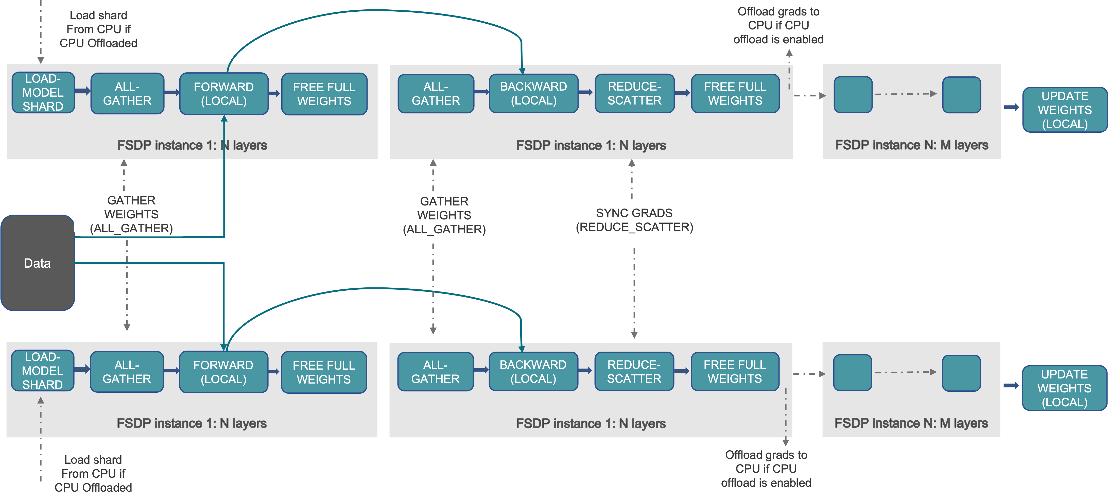
• Fully Sharded Data Parallel (FSDP)
  • FSDP is an advanced form of data parallelism designed to significantly reduce the memory footprint on each GPU. Instead of replicating everything in DP, FSDP shards (partitions) the model’s parameters, gradients, and optimizer states across the data-parallel processes (GPUs). Each GPU only holds of slice of these components, lowering per-GPU memory requirements.

And several other techniques that are used in combining Data and Model,

The following table, quickly summarize the above parallelism techniques,

We will focus on the Data Parallelism technique specifically DistributedDataParallel (DDP) which enables large-scale deep learning training.

DataParallel vs DistributedDataParallel

The DataParallel module in PyTorch is a single process, multi-threaded approach that only works on a single machine. Although it can utilize multiple GPUs, it has limitations due to Python’s Global Interpreter Lock (GIL). The GIL ensures that only one thread executes Python bytecode at a time, even on multi-core processors. As a result, DataParallel often becomes a performance bottleneck and is relatively slow compared to DistributedDataParallel (DDP), even in single-GPU setups.

In contrast, DDP is a multi-process approach that supports both single and multi-GPU training. Each process is assigned to a single GPU, which is the recommended practice to spawn 1 process: 1 GPU. This avoids contention in CUDA streams and simplifies NCCL topology detection, leading to better performance and stability.

DataParallel, is a single-process, multi-threaded but it can work only in single machine. Approaches using concurrent processes and multi-processing library are used to make max use of the available GPU resources. However, DistributedDataParallel is multi-process and supports both single and multi gpu training. Due to Global Interpreter Lock (GIL) in Python which is a locking mechanism that ensures only one thread can execute python bytecode at a given time even on multi-core processors. As a results DataParallel is relatively slow compared to DistributedDataParallel even on single-gpu training setup. This is a huge setback in DataParallel, making DDP as the go-to choice for distributed training.  DP, on the other hand, becomes less efficient with a larger number of GPUs because it involves a bottleneck in synchronizing gradients using a single process, making it harder to scale efficiently.

Why prefer DDP?

• DataParallel replicates the model across multiple GPUs, but uses a single process to aggregate gradients. This results in inefficient scaling, especially with a larger number of GPUs.
• DDP, by spawning separate processes per GPU, avoids CUDA stream contention and enable each process to have dedicated and reliable access to its GPU.
• During training, DDP registers an autograd hook for each model parameter. When the backward pass is executed, these hooks trigger gradient synchronization across all processes. This ensures that all processes compute the same updated gradients and remain in sync throughout training.

Best Practices in DDP

• In multi-node setups, ensure identical environments in both nodes, for example with docker containers.
• Checkpoint the model regularly and ensure only one process handles saving.
• Robust network connectivity between all nodes.
• Regularly check GPU utilization and use profiler to identiy and resolve any bottlenecks.
• All processes must agree on rank assignments, Training will freeze if the master node is incorrectly set which is typically Rank 0.
• The master node needs SSH key-based password-less access to all worker nodes for proper communication in a multi-node training.
• Set seed for reproducibility.

Click here to download the source code to this post

Code Walkthrough of Single Node Multi-GPU Setup in Kaggle T4x2

Let’s put our learnings into practice. For this experiment we will train a ResNet-18 model on the CIFAR10 dataset using DDP. We will use torch.multiprocessing.spawn to launch multiple process each controlling only one GPU.

Import Dependencies

%%writefile train.py

import os
import time
import datetime

import torch
import torch.nn as nn
import torch.optim as optim
from torch.optim import lr_scheduler
import torch.backends.cudnn as cudnn

import torchvision
import torchvision.transforms as transforms
from torchvision.datasets import CIFAR10
from torch.utils.data import DataLoader

import torch.distributed as dist
import torch.multiprocessing as mp
import torch.utils.data.distributed

# from model import pyramidnet
import argparse
from tensorboardX import SummaryWriter

We will use the NCCL library as the backend with a TCP store for initialization. Since Kaggle’s T4x2 instances are part of single node, the world_size is 2 * 1 = 2. The ranks for two GPUs are 0 and 1 respectively.

parser = argparse.ArgumentParser(description='cifar10 classification models')
parser.add_argument('--lr', default=0.1, help='')
parser.add_argument('--resume', default=None, help='')
parser.add_argument('--batch_size', type=int, default=768, help='')
parser.add_argument('--num_workers', type=int, default=4, help='')
parser.add_argument("--gpu_devices", type=int, nargs='+', default=None, help="")

parser.add_argument('--gpu', default=None, type=int, help='GPU id to use.')
parser.add_argument('--dist-url', default='tcp://127.0.0.1:3456', type=str, help='')
parser.add_argument('--dist-backend', default='nccl', type=str, help='')
parser.add_argument('--rank', default=0, type=int, help='')
parser.add_argument('--world_size', default=1, type=int, help='')
parser.add_argument('--distributed', action='store_true', help='')
args = parser.parse_args()

gpu_devices = ','.join([str(id) for id in args.gpu_devices])
os.environ["CUDA_VISIBLE_DEVICES"] = gpu_devices

Next, simply load the pretrained resnet18 with imagenet weights and modify its last linear head for transfer learning. The model is defined globally, so each spawn process can get a copy of this initial model definition.

model = torchvision.models.resnet18(weights = 'DEFAULT')
model.fc = nn.Linear(model.fc.in_features, 10)

# summary(model, (1, 3, 224, 224), device = "cpu")
# model.to(device) # move to gpu
print("--- Model Loaded --- ")

The main() is the core launching mechanism in which torch.multiprocessing.spawn will create ngpus_per_node new processes to run parallely by inferring the local rank . Each new process will execute the main_worker function.

def main():
    args = parser.parse_args()

    ngpus_per_node = torch.cuda.device_count()

   # total processes that participates in the training.
    args.world_size = ngpus_per_node * args.world_size
    mp.spawn(main_worker, nprocs=ngpus_per_node, args=(ngpus_per_node, args))
  

Then process group is initialized and each spawned process is assigned a GPU and set it as the active CUDA device.

 def main_worker(gpu, ngpus_per_node, args):
    args.gpu = gpu
    ngpus_per_node = torch.cuda.device_count()    
    print("Use GPU: {} for training".format(args.gpu))
        
    args.rank = args.rank * ngpus_per_node + args.gpu    
    dist.init_process_group(backend=args.dist_backend, init_method=args.dist_url,
                            world_size=args.world_size, rank=args.rank)

    print('==> Making model..')
    net = model
    torch.cuda.set_device(args.gpu)
    net.cuda(args.gpu)
    args.batch_size = int(args.batch_size / ngpus_per_node)
    args.num_workers = int(args.num_workers / ngpus_per_node)

After loading and moving the model to the assigned GPU, it’s wrapped with DistributedDataParallel (DDP) which:

• Handles gradient synchronization between processes.
• Ensures each GPU computes on different data slices.

We also need to prepare the data in a way that’s complies with the distributed network setup by sharding the data using DistributedSampler. This ensures that each process receives a unique subset of the dataset, with no data overlap across GPUs.

 def main_worker(gpu, ngpus_per_node, args):
    .   .   . 
    net = torch.nn.parallel.DistributedDataParallel(net, device_ids=[args.gpu])
    num_params = sum(p.numel() for p in net.parameters() if p.requires_grad)
    print('The number of parameters of model is', num_params)

    print('==> Preparing data..')
    transforms_train = transforms.Compose([
        transforms.RandomCrop(32, padding=4),
        transforms.RandomHorizontalFlip(),
        transforms.ToTensor(),
        transforms.Normalize((0.4914, 0.4822, 0.4465), (0.2023, 0.1994, 0.2010))])

    dataset_train = CIFAR10(root='./data', train=True, download=True, 
                            transform=transforms_train)
    train_sampler = torch.utils.data.distributed.DistributedSampler(dataset_train)
    train_loader = DataLoader(dataset_train, batch_size=args.batch_size, 
                              shuffle=(train_sampler is None), num_workers=args.num_workers, 
                              sampler=train_sampler)

    # there are 10 classes so the dataset name is cifar-10
    classes = ('plane', 'car', 'bird', 'cat', 'deer', 
               'dog', 'frog', 'horse', 'ship', 'truck')
    
    criterion = nn.CrossEntropyLoss()
    optimizer = optim.SGD(net.parameters(), lr=args.lr, 
                          momentum=0.9, weight_decay=1e-4)
    
    train(net, criterion, optimizer, train_loader, args.gpu)
            

The train function looks similar to the standard non-distributed training loop. The forward pass is local, however, during loss.backward(), DDP’s internal hooks automatically trigger an all_reduce operation across all process in the group to sum and sync the gradients for each parameter. When optimizer.step() is called, each process independently updates its local copy of the model parameters. Since they all started with the same parameters (synchronized by DDP during initialization) and apply the same averaged gradients, the model replicas remain in sync.

Final Gradient (G) = All Reduce(Gradient 1, Gradient 2,..., Gradient n)

def train(net, criterion, optimizer, train_loader, device):
    net.train()

    train_loss = 0
    correct = 0
    total = 0
    
    epoch_start = time.time()
    for batch_idx, (inputs, targets) in enumerate(train_loader):
        start = time.time()
        
        inputs = inputs.cuda(device)
        targets = targets.cuda(device)
        outputs = net(inputs)
        loss = criterion(outputs, targets)

        optimizer.zero_grad()
        loss.backward()
        optimizer.step()

        train_loss += loss.item()
        _, predicted = outputs.max(1)
        total += targets.size(0)
        correct += predicted.eq(targets).sum().item()

        acc = 100 * correct / total
        
        batch_time = time.time() - start
        
        if batch_idx % 20 == 0:
            print('Epoch: [{}/{}]| loss: {:.3f} | acc: {:.3f} | batch time: {:.3f}s '.format(
                batch_idx, len(train_loader), train_loss/(batch_idx+1), acc, batch_time))
    
    elapsed_time = time.time() - epoch_start
    elapsed_time = datetime.timedelta(seconds=elapsed_time)
    print("Training time {}".format(elapsed_time))
    

if __name__=='__main__':
    main()

Inorder, for distributed training to work as expected, it’s recommended to run the script as a .py rather than in jupyter cells.

# For Kaggle T4x2 So we pass two ids
!python train.py --gpu_device 0 1  --batch_size 768 --epochs 5

--- Model Loaded --- 
--- Model Loaded --- 
Use GPU: 1 for training
--- Model Loaded --- 
Use GPU: 0 for training
==> Making model..
==> Making model..
The number of parameters of model is The number of parameters of model is11181642 
11181642==> Preparing data..

==> Preparing data..
Files already downloaded and verifiedFiles already downloaded and verified

--- Model Loaded --- 
--- Model Loaded --- 
--- Model Loaded --- 
--- Model Loaded --- 
Epoch: [0/66]| loss: 2.560 | acc: 11.458 | batch time: 0.807s 
Epoch: [0/66]| loss: 2.609 | acc: 13.802 | batch time: 0.931s 
Epoch: [20/66]| loss: 2.093 | acc: 34.772 | batch time: 0.095s 
Epoch: [20/66]| loss: 2.130 | acc: 34.338 | batch time: 0.092s 
Epoch: [40/66]| loss: 1.876 | acc: 42.124 | batch time: 0.096s Epoch: [40/66]| loss: 1.819 | acc: 42.537 | batch time: 0.093s 

. . .
Epoch: [20/66]| loss: 1.708 | acc: 37.140 | batch time: 0.102s 
Epoch: [20/66]| loss: 1.675 | acc: 38.777 | batch time: 0.108s 
Epoch: [40/66]| loss: 1.636 | acc: 39.685 | batch time: 0.104s 
Epoch: [40/66]| loss: 1.665 | acc: 38.523 | batch time: 0.102s 
Epoch: [60/66]| loss: 1.611 | acc: 40.450 | batch time: 0.099s 
Epoch: [60/66]| loss: 1.625 | acc: 40.027 | batch time: 0.115s 
Training time per epoch 0:00:32.473986
Training time per epoch 0:00:32.477097

Conclusion

With PyTorch’s excellent support for distributed training, it’s now more accessible to scale deep learning workloads without any hassle. In this article, we briefly explored the fundamentals of Distributed Data Parallel (DDP) and other key concepts along with a simple training experiment in Kaggle T4x2.

We can extend this knowledge to setup multi-node GPU setups which enables even larger and faster model training pipelines.

References

1. PyTorch Multi GPU Implementation
2. Multi-node Distributed Training
3. A Gentle Introduction to DDP: Medium