CVPR 2024: An Overview and Key Papers

AI research made great strides in 2023-2024, including VLLMs like GPT4-O and Gemini; Text-to-Video Diffusion Models like SORA and Veo; and Humanoids like Atlas V2, Figure -01, and Tesla Optimus. Extensive research is ongoing every day behind all of these latest innovations. To showcase the best research in this rapid advancement in AI, the IEEE Computer Society (CS) and the Computer Vision Foundation (CVF) organize CVPR (CVPR 2024), the world’s best conference for showcasing the latest research in Computer Vision and AI.

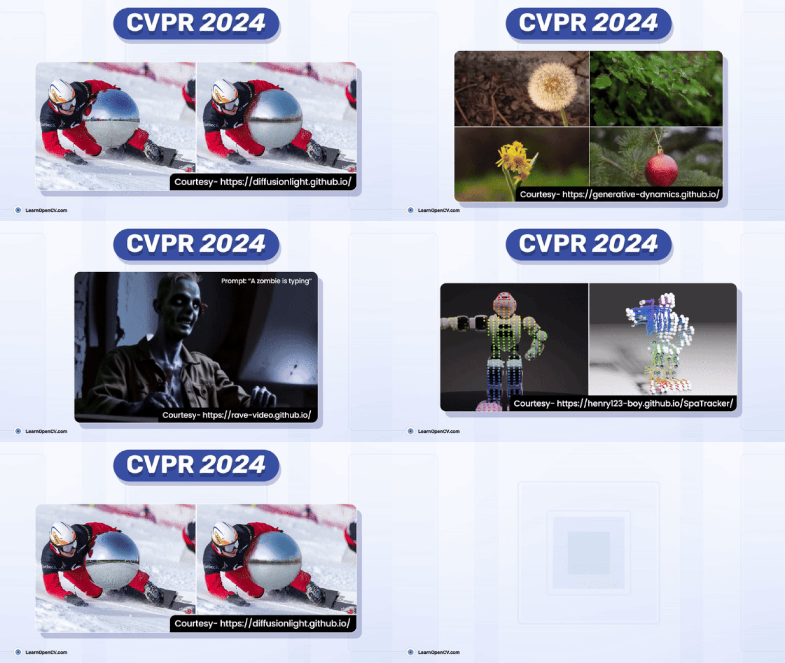
According to a survey by Express Computer, about 13.5K papers are published daily, and approximately 550 papers are published every hour. In 2024, CVPR was conducted from June 17th to 21st in Seattle, and we witnessed some cool research happening around the globe. In this article, we try to cover some of the research papers that caught our attention. By the end of this article, you will have an overview of CVPR and the latest research going on advanced Computer Vision and AI around the world. 

OpenCV at CVPR 2024

Gary Bradski, Anindya Roy, Phil Nelson, and ShiQi Yu represented the OpenCV team at CVPR 2024. Here are some key highlights that the team showcased at booth 1920:

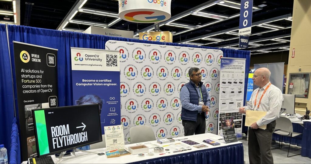
1. The Team featured OpenCV 5, showcasing features from the latest releases and roadmap for OpenCV 5. At last count, 600+ attendees added themselves to OpenCV’s visitor list. 
2. Everybody thanked the developers of OpenCV for making many graduate courses, MS/PhD projects, and commercial solutions possible. A handful of industry attendees promised support via memberships.
3. The Team highlighted OpenCV University and OpenCV.ai to educate people about the latest AI and Computer Vision.
4. Several representatives from semiconductor and camera companies, impressed by recent collaborations with Arm and Qualcomm, have invited OpenCV to join their partnership programs.
5. MLOps and CV tooling teams like Voxel51 requested collaborations. 

Paper 1: Generative Image Dynamics

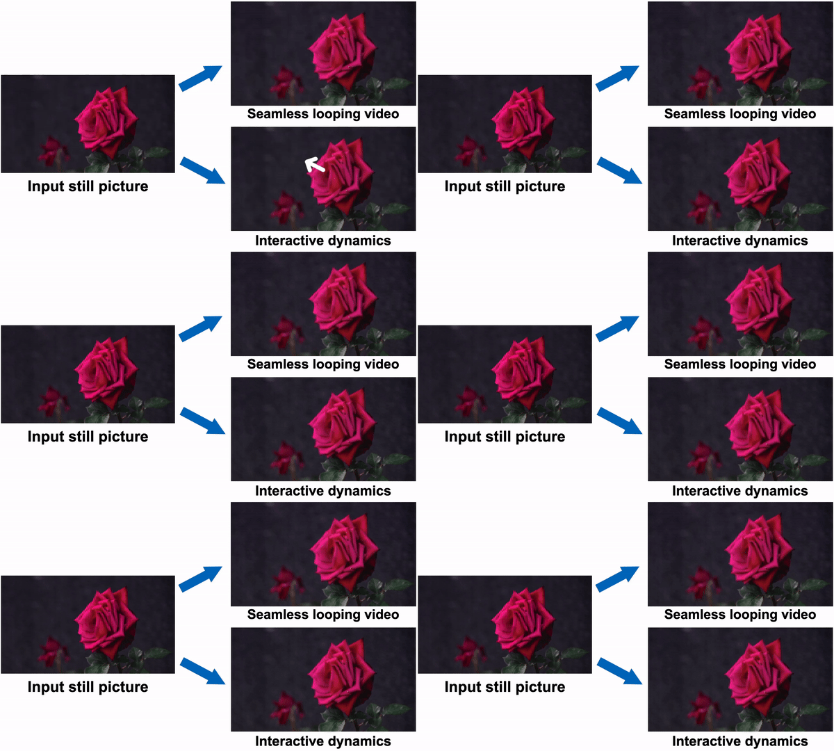
A paper by Zhengqi Li, Richard Tucker, et al. from Google Research got the best paper award at CVPR 2024. This paper is all about generating a seamlessly looping video or an interactive simulation of dynamics from a single image. The model trained on a collection of motion trajectories extracted from real video sequences depicting natural, oscillatory dynamics of objects such as trees, flowers, candles, and clothes swaying in the wind.

Now, if you give a single image to the model, it will use a frequency-coordinated diffusion sampling process to predict a spectral volume, which can be converted into a motion texture that spans an entire video. Along with an image-based rendering module, the predicted motion representation can be used for a number of downstream applications, such as turning still images into seamlessly looping videos, or allowing users to interact with objects in real images, producing realistic simulated dynamics (like dragging and releasing points).

Model Architecture

Motion prediction module: The model predicts a spectral volume S through a frequency-coordinated denoising model. Each block of the diffusion network θ interleaves 2D spatial layers with attention layers (red box, right), and iteratively denoises latent features zⁿ . The denoised features are fed to a decoder D to produce S. During training, the model concatenates the downsampled input I₀ with noisy latent features encoded from a real motion texture via an encoder E, and replaces the noisy features with Gaussian noise z^N during inference (left).

Predicting Motion

Motion Representation

• Concept: A “motion texture” comprises sequences of time-variant 2D displacement maps F_t, where each map specifies the displacement of pixels in an input image I₀ over time t.
• Implementation: We pass the image I₀ and replace the noisy features with Gaussian noise z^N to the model. The model predicts the spectral volumes(S) using reverse diffusion.
• Spectral Volume Representation: Motions are encoded in the frequency domain by transforming per-pixel trajectories into spectral volumes using a Fourier transform. This allows complex motion dynamics to be represented compactly and processed efficiently.

Predicting Motion with a Diffusion Model

• Latent Diffusion Model (LDM): Chosen for its computational efficiency and the ability to maintain synthesis quality. The model consists of:
  • Variational Autoencoder (VAE): This component compresses the input image into a latent space and reconstructs the input from these features.
  • U-Net-Based Diffusion Model: It learns to iteratively denoise latent features, starting from Gaussian noise, producing spectral volumes through denoising steps.
• Training and Normalization:
  • Frequency Adaptive Normalization: Critical in preparing the data for the model, this step normalizes the Fourier coefficients to prevent extremes by using statistics (like the 95th percentile) from training data.
  • Motion Prediction: Utilizes the trained model to predict spectral volumes by applying a frequency-coordinated denoising process. This method ensures that predictions across frequency bands are harmonized, avoiding unrealistic motion artifacts.

Image-Based Rendering

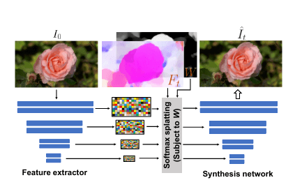
Rendering module: The method fills in missing content and refines the warped input image using a deep image-based rendering module, where multi-scale features are extracted from the input image I. Softmax splatting is applied over the features with a motion field F_t from 0 to t (subject to the weights W). The warped features are fed to an image synthesis network to produce the rendered image I_t.

• Forward Warping: This involves transforming the predicted motion texture back into a time domain using inverse FFT and then using this texture to warp the input image into a new frame I_t.
• Softmax Splatting:
  • Technique: Used for refining the warped image by blending multiple source pixels that map to the same output location. This is achieved using a feature pyramid and softmax weights to manage overlapping and smooth transitions.
  • Implementation: The image I₀ is encoded into multi-scale feature maps. The motion field F_t is applied to these features, which are then synthesized into the output image I_t using a neural synthesis network.

• Perceptual Loss: During training, a perceptual loss based on the VGG network compares the synthesized frames against actual video frames to fine-tune the model’s output for higher fidelity and realism.

Examples

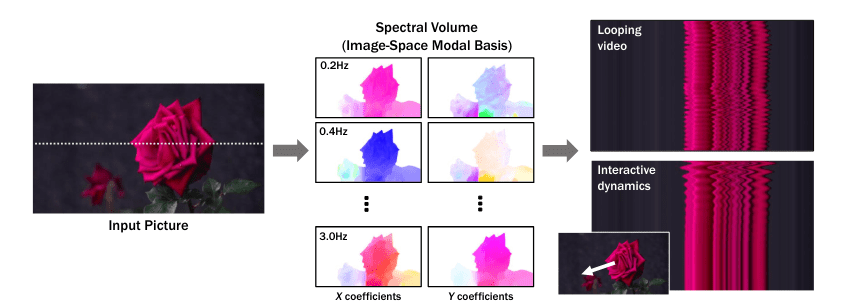
Image-to-Video Conversion

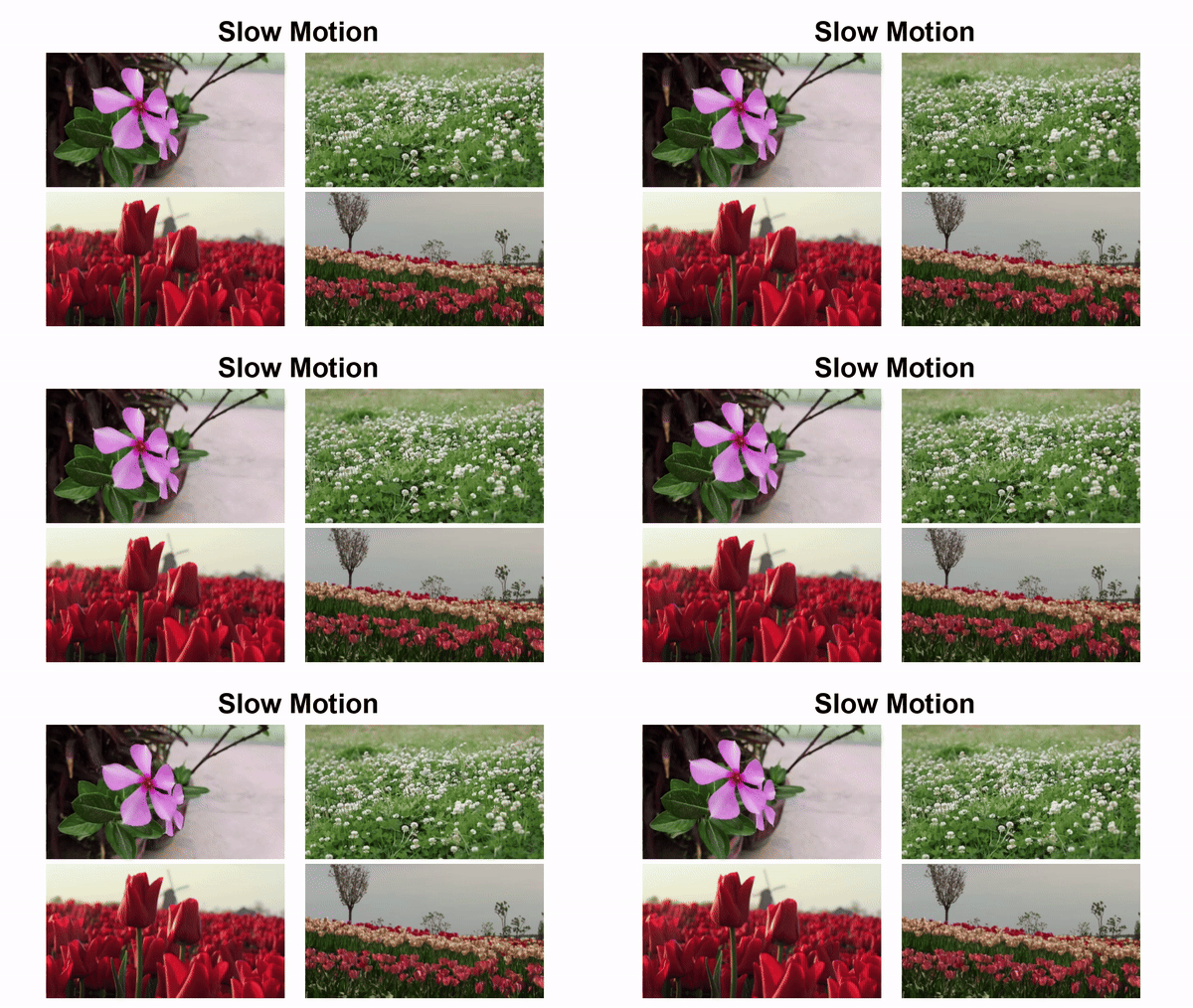
• Basic Idea: The model transforms a single still photo into a dynamic video by first calculating a “motion spectral volume” from the photo. This volume captures all possible movements in the scene.
• Animation Process: Then, these calculated motions are turned into a smooth video using a special module. 

Seamless Looping Videos

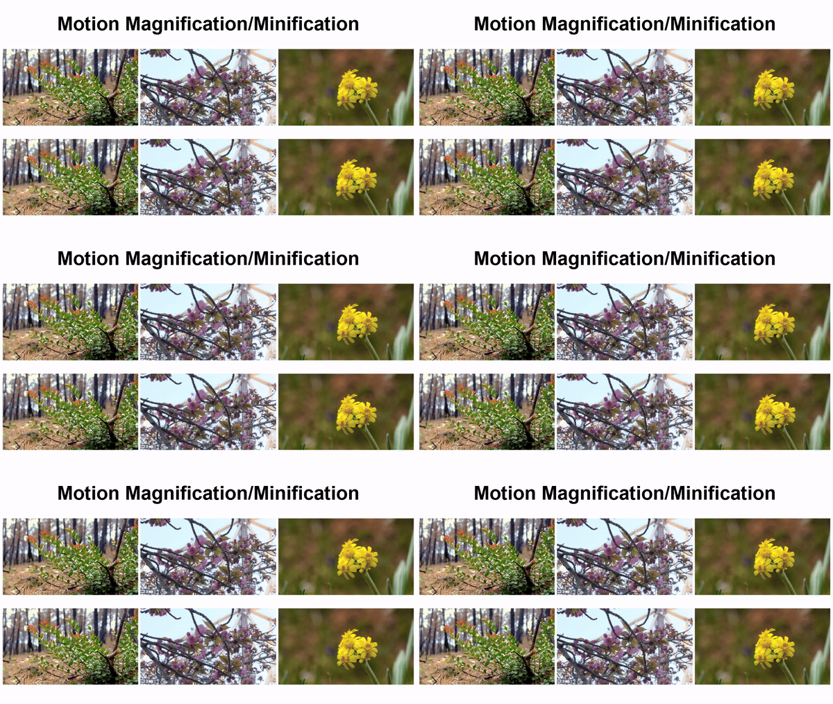
• Challenge: Looping videos are those that start and end at the same point smoothly, so they can run continuously without you noticing the beginning or end. Creating these types of videos is challenging because it’s hard to find examples to teach the model.
• Solution: The authors developed a technique using a motion prediction model that ensures the start and end of the video match up perfectly. This involves a clever trick where they tweak the model during the video creation process to focus on making the start and end frames look the same. During the video-making process, each pixel’s movement is adjusted to make the first and last frames nearly identical, making the video loop seamless.

Interactive Dynamics from a Single Image

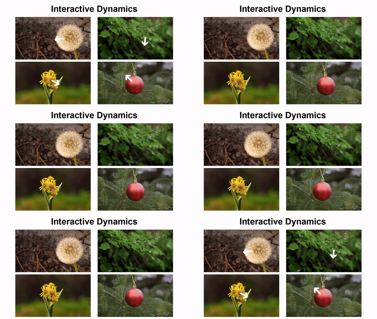
• Concept: This technique allows us to make a still photo react to virtual forces, like poking or pushing an object in the photo, and see it move realistically.
• How It Works: We use a special mathematical model that mimics real-world physics. By assigning different frequencies to movements in the image, we can predict how each part should move in response to a force based on how objects naturally vibrate.
• Application: This can be particularly useful in simulations or interactive applications where you want to create realistic movements without needing actual video footage as input.

Our Take

• The paper is unique in introducing a frequency-coordinated diffusion sampling process to predict a spectral volume from a single image.
• We like how it uses diffusion to generate motion frequencies from an image.
• The authors haven’t released the code yet, but you can try the demo here.

Paper 2: Hydra-MDP: End-to-end Multimodal Planning with Multi-target Hydra-Distillation

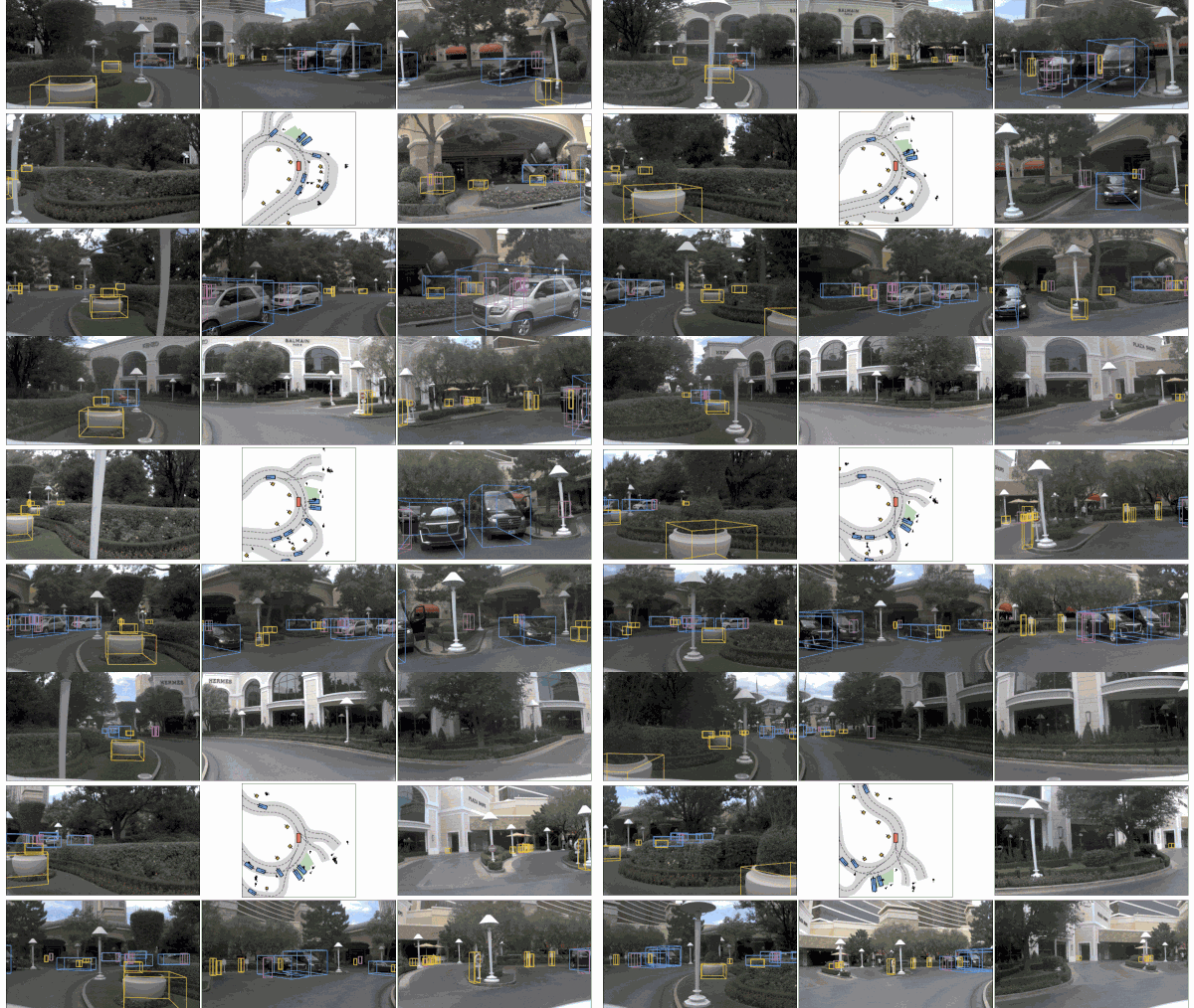
Traditional autonomous vehicle(AV) systems are built upon many steps, such as detection, tracking, trajectory detection, and path planning. Zhenxin Li, Kailin Li, Shihao Wang, et al. at Nvidia research, introduce Hydra-MDP, an end-to-end driving system for perception and decision-making under a unified transformer model. With this model, Nvidia won the CVPR Autonomous Grand Challenge for End-to-End Driving this year.

After Using the Hydra-MDP, the researcher made better predictions with less code and less complicated architecture. They introduced the transformer-based model, which takes over traditional deep learning network systems, outperforms all the prior methods, and won the CVPR Grand Challenge. They also introduced another notable work called Producing and Leveraging Online Map Uncertainty in Trajectory Prediction, which is one of the main part of the Hydra Pipeline.

Many online HD vector map estimation methods operate by encoding multi-camera images, transforming them to a common BEV feature space, and regressing map element vertices. This work augments the common output structure with a probabilistic regression head, modeling each map vertex as a laplace distribution. To access the resulting downstream effects, researchers further extend downstream prediction models to encode map uncertainty, augmenting both GNN-based and Transformer-based map encoders.  You can read the above-mentioned paper for more detailed explanations.

After using this method and Hydra-MDP together, the research not only generated a better HD map but also improved overall AV system performance. Now, let’s move to the main architecture of Hydra-MDP.

Architecture Overview

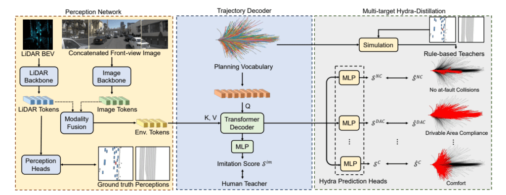
Perception Network:

• The model takes two inputs: a 2D image from a multiview camera and a LiDAR Bird’s Eye View depth map from a LiDAR sensor. 
• Then, we pass both the inputs through an image Backbone and a LiDAR backbone separately. These backbone encoders generate embeddings for both the inputs.
• Then, the model does a modality fusion between these two different modality embeddings (2D and 3D), and generates new environment embeddings.
• Simultaneously, the model passes the LiDAR tokens to a Perception Head to predict the ground-truth perceptions. The model uses these data later to predict the perfect trajectory path for the AV.

Trajectory Decoder:

• In this part, the model uses a Planning Vocabulary (data containing all the possible trajectory paths for a vehicle that can move in an environment) to generate query embeddings (Q) using another encoder.
• Later, this Query (Q) is passed with Key (K) and Value (V) in a transformer decoder block.
• After moving into the decoder block, it goes into the MLP block, which yields imitation scores for each video frame embedding.
• With these imitation scores, the model starts learning with the Human Teacher model (this is data collected from human drivers. It includes things like the paths they take (trajectories), how they handle different driving situations when they brake, accelerate, turn, etc.), which calculates a distance-based cross-entropy loss value for each to imitate human drivers.
• Finally, the model considers the trajectory proposals that are close to human driving behaviors from a probability distribution using softmax applied to L2 distances.

Multi-target Hydra-Distillation:

• We use the model to simulate the trajectory paths for the AV in a virtual environment (think of it as a 3D simulation environment) and train the model according to it. 
• It takes the output embeddings from the transformer block and passes those to Hydra Prediction Heads (a layer made of multiple MLP blocks), which give three sets of imitation scores.
• Simultaneously, we use the planning vocabulary with the ground truth perceptions in a simulator with rule-based teachers. The rule-based teacher uses simulations to generate many driving scenarios. 
• For each simulated driving path, the rule-based teacher gives scores based on how well the driving adheres to various safety and rule-based criteria. These scores are about avoiding collisions, staying within the drivable area, how comfortable the ride is, etc. These scores act like feedback for the student model, showing how well it performed according to the rules.
• Rule-based teachers generate scores for different trajectories by running detailed simulations. These scenarios include:
  • No at-fault Collisions (SNC) – In this case, there is a collision, but it is not the fault of the AV.
  • Drivable Area Compliance (SDAC) – Keeping the car on the correct part of the road according to the traffic rules.
  • Comfort (SC) – Ensuring the ride is smooth without any sudden jerks or harsh movements.
• Now, the most interesting part: the model uses the simulator with the rule-based teacher approach to generate the simulations for each trajectory path of these three sets of scores.
• Then, during training, the model optimizes the imitation scores generated from the Hydra prediction heads with the generated simulation scores(with the trajectory paths) from rule-based teachers.
• At the time of inference, the prediction head predicts the imitation score that is later simulated into the trajectory paths. The AV finally uses these predicted trajectory paths to navigate through the environment.

Code 

The authors haven’t released the codebase yet. You can check the official GitHub repo here to have an update.

Paper 3: pixelSplat: 3D Gaussian Splats from Image Pairs for Scalable Generalizable 3D Reconstruction

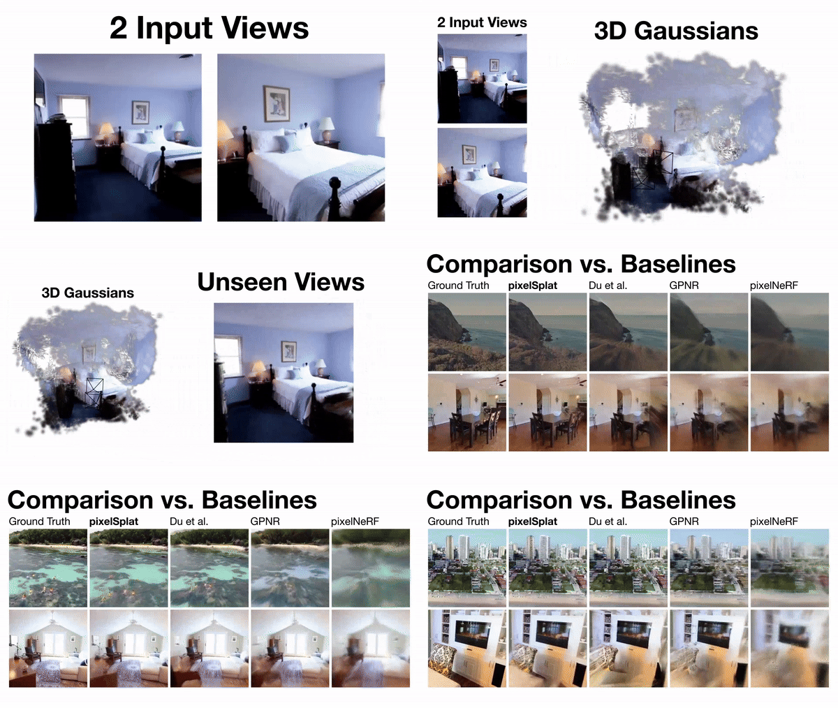
Over the past two decades, the term “3D” has been way too popular in AI research. 3D reconstruction is one of the most popular research areas in computer vision. We all know about the groundbreaking paper NeRF, which introduced the neural network to generate 3D renders. Then we got pixelNeRF, which uses only a few images as input, and a CNN-based Encoder on top of NeRF to generate far better 3D renders. And then, we have 3D Gaussian Splatting, which uses 3D Gaussian and gradient descent to generate better 3D renders than priors. 

Authors David Charatan, Sizhe Lester Li, et al. take this research a step ahead and introduce pixelSpat, which combines 3D Gaussian splatting with a reparameterization trick and a neural network. It takes just two images of an object from two different viewpoints and generates a 3D render within minimal inference time. We can think of this approach as a combination of 3D Gaussian Splatting and NeRF. 

Architecture Overview

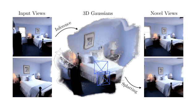
• Two-View Image Encoding: PixelSplat begins by processing a pair of input images through a feature extraction network, which generates a high-dimensional representation of each image. This neural network, often structured similarly to those used in NeRF architectures, extracts crucial visual and spatial features from the images, setting the stage for understanding the scene’s geometry.
• Epipolar Geometry and Scale Ambiguity Resolution: The extracted features are then processed using an epipolar transformer, a component that leverages the geometric relationship between the two views to resolve scale ambiguity—an inherent challenge in reconstructing 3D scenes from 2D images. This step ensures that the 3D positions inferred from different images are consistent relative to each other, addressing variations in camera positioning and orientation.

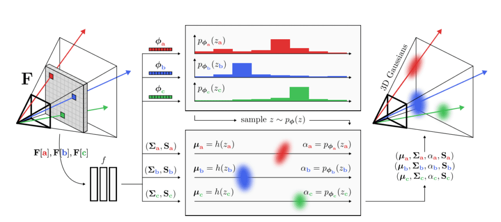
• Probabilistic Sampling of Gaussian Parameters: With scale and geometry calibrated, the next step involves a novel application of 3D Gaussian splatting, where the model predicts a dense probability distribution for the potential locations of Gaussian primitives. This approach is facilitated by the reparameterization trick, which allows the network to sample these locations differently. Here, each Gaussian’s position (mean), shape (covariance), and visibility (opacity) are determined, enabling gradients to be propagated back through the network during training, thus optimizing the Gaussian placement efficiently.
• Rendering and Output Generation: Finally, the parameterized 3D scene, now represented as a collection of Gaussian splats, is rendered to produce novel views. This rendering process is optimized for speed and memory efficiency, making use of the Gaussian splatting technique’s light computational footprint. The output is a set of new images, or novel views, generated from perspectives not originally captured by the input images, showcasing the model’s ability to interpolate and extrapolate 3D space from limited data.

More Examples

ACID Dataset

Real Estate 10k Dataset

Code Walkthrough

First, go to the official GitHub repo mentioned above, then clone the repo:

git clone https://github.com/dcharatan/pixelsplat.git

Then, create a virtual environment and install all the required libraries:

python3.10 -m venv ven
source venv/bin/activate
# Install these first! Also, make sure you have python3.11-dev installed if using Ubuntu.
pip install wheel torch torchvision torchaudio
pip install -r requirements.txt

Then, download and place the model checkpoints and dataset from the official GitHub repository.

And you are good to go. So, it uses Hydra, a framework by Meta, which uses a different set of arguments:

# Real Estate 10k
python3 -m src.main +experiment=re10k mode=test dataset/view_sampler=evaluation dataset.view_sampler.index_path=assets/evaluation_index_re10k.json checkpointing.load=checkpoints/re10k.ckpt
# ACID
python3 -m src.main +experiment=acid mode=test dataset/view_sampler=evaluation dataset.view_sampler.index_path=assets/evaluation_index_acid.json checkpointing.load=checkpoints/acid.ckpt

Paper 4: Visual Anagrams: Generating Multi-View Optical Illusions with Diffusion Models

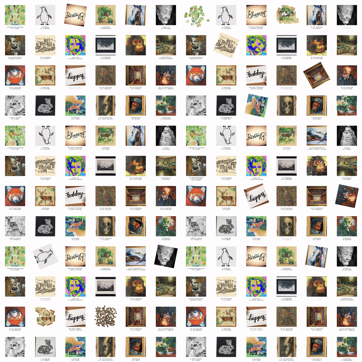
In computer vision, we always have this concept called illusions, such as checker shadow illusions, but have you ever thought that we can use diffusion to create multiview illusion images? Cool right!

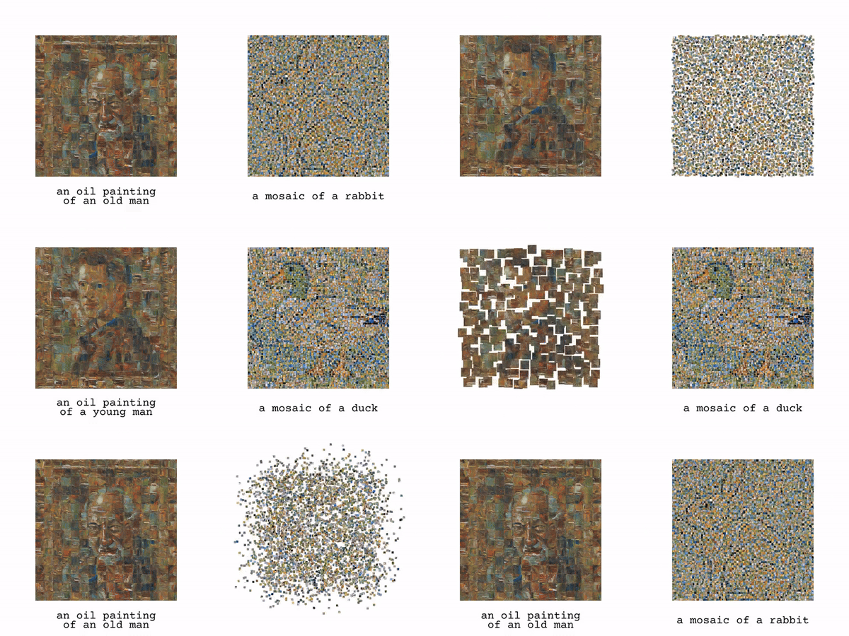
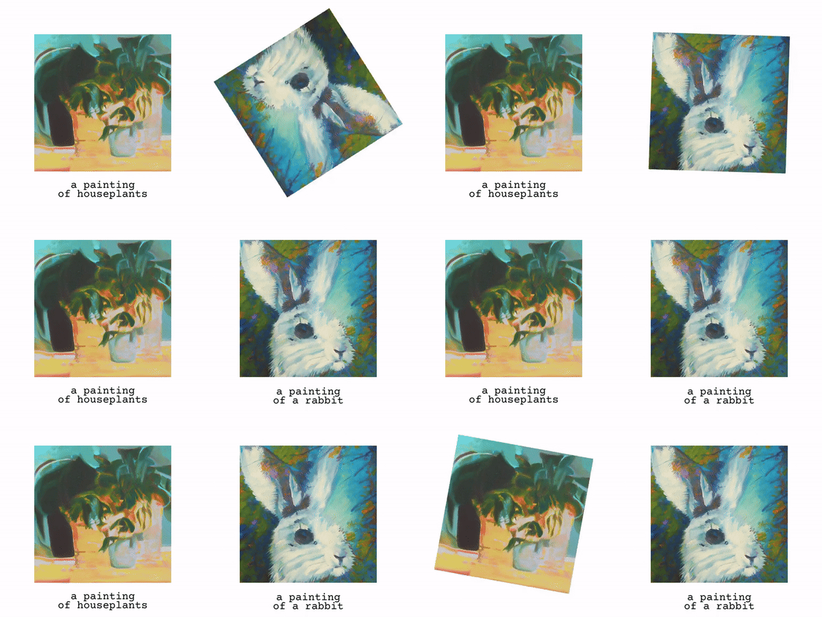
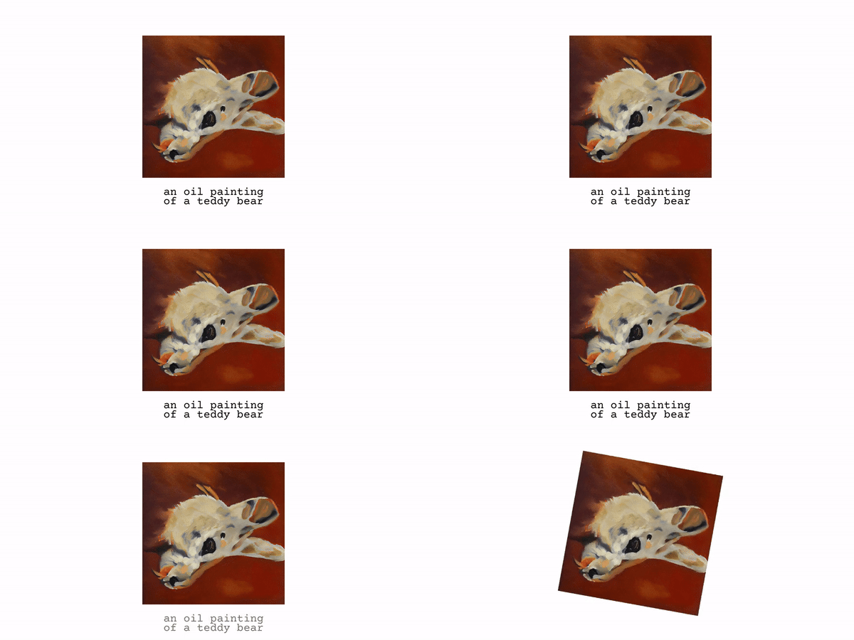
Authors Daniel Geng, Inbum Park, and Andrew Owens proposed Visual Anagram, a method that uses diffusion to create any kind of visual illusion image with simple prompts. It not only creates the illusion image but also supports a wide range of transformations, including rotations, flips, color inversions, skews, jigsaw rearrangements, random permutations, and multiple views.

Method Overview

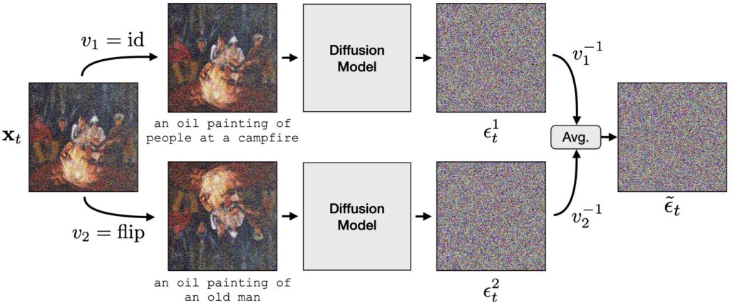
• First, it takes the input image, passes it to the diffusion model with a prompt, and performs simple reverse diffusion.
• The interesting part is that it parallelly takes a transformation of that image, for example, the identity function, an image flip, or a permutation of pixels, and passes that to the diffusion model with another prompt.
• After we get the noise estimates, the model simply takes the average of those noise estimates and denoises it to get the final illusion image.

More Examples

Jigsaw Permutations

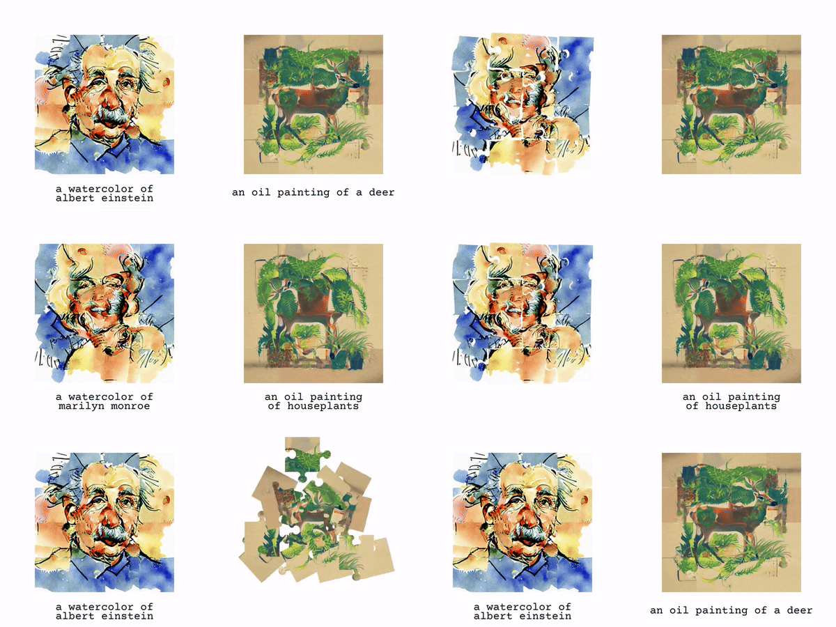
Flips and 180° Rotations

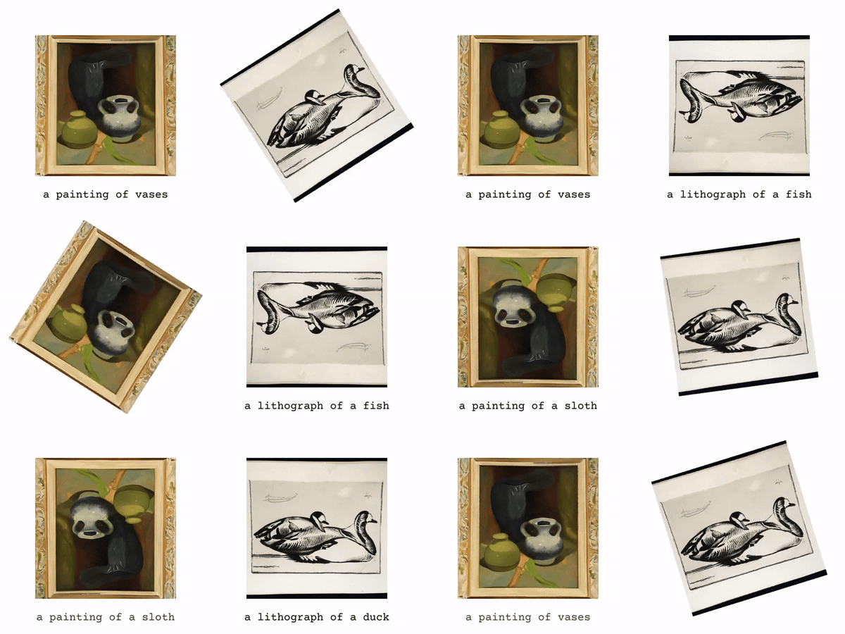
90° Rotations

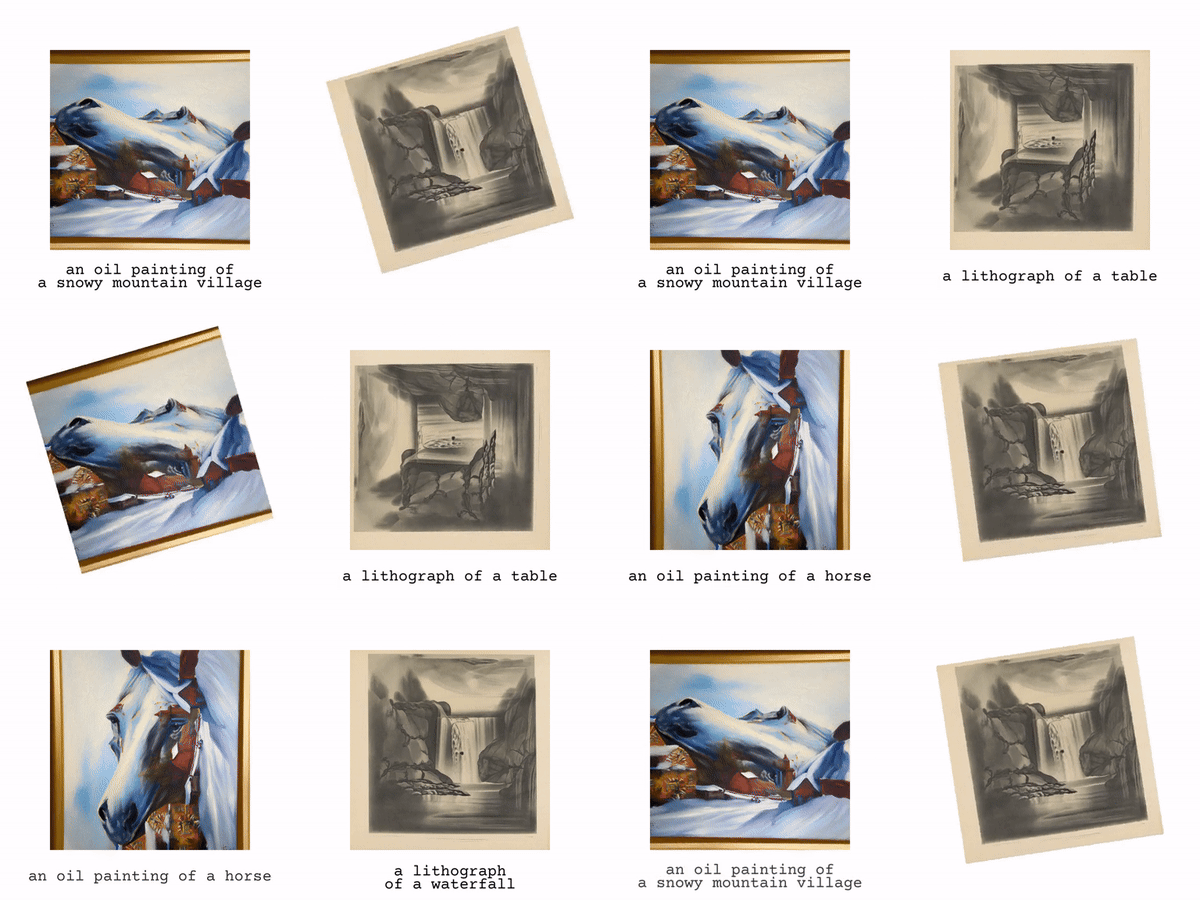
Color Inversions

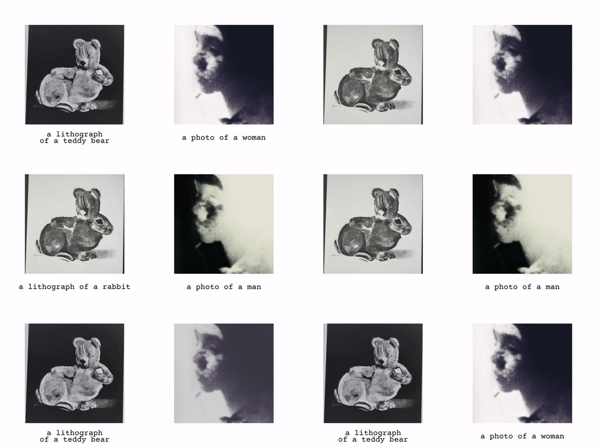
Miscellaneous Transformations

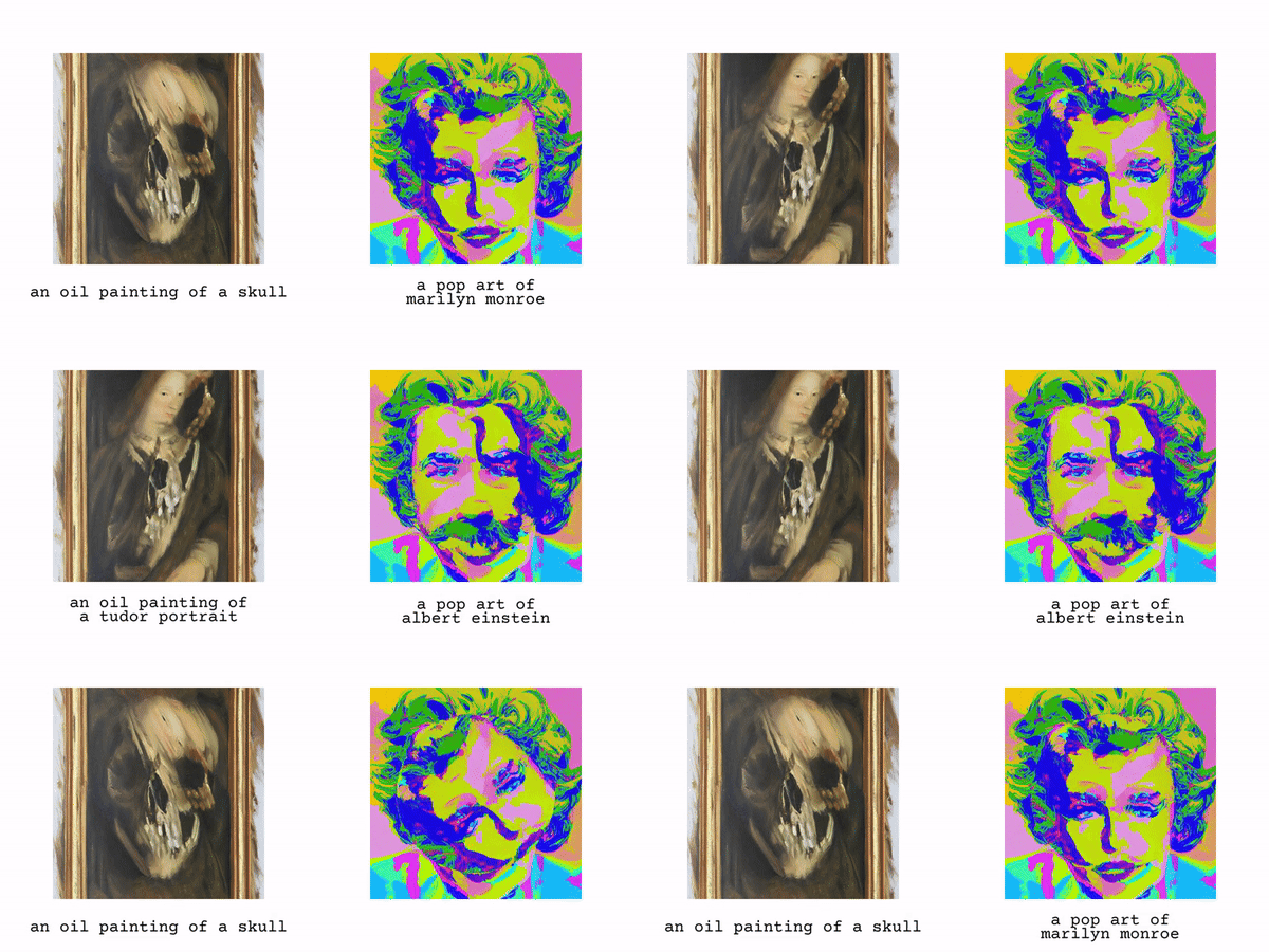
Random Patch Permutations

Three Views

Four Views

Code Pipeline

Authors have provided the Colab NoteBooks, both the free and pro tier. 

If you want to use it locally, follow the instructions at the GitHub mentioned above.

Paper 5: RAVE: Randomized Noise Shuffling for Fast and Consistent Video Editing with Diffusion Models

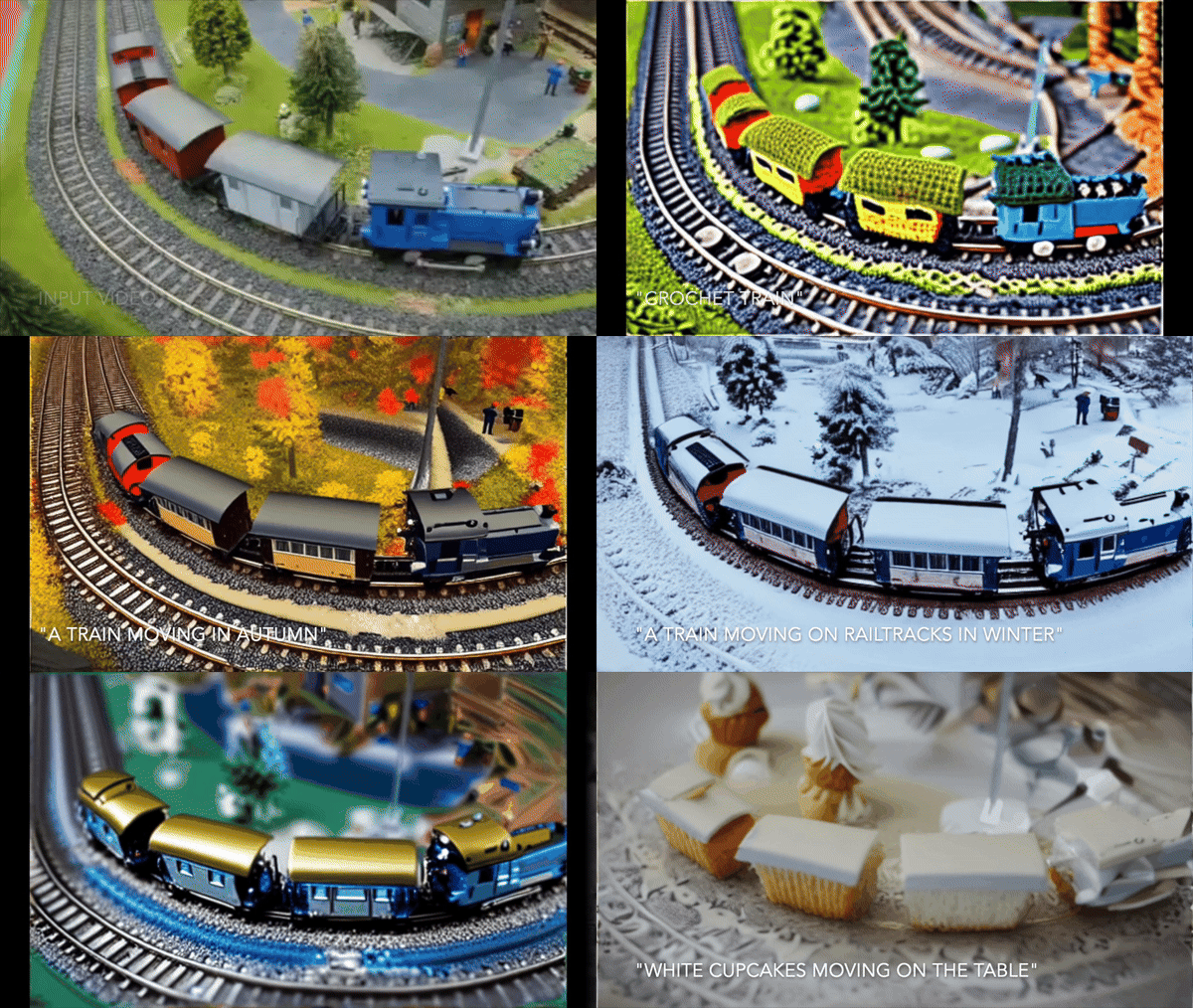
This CVPR, Ozgur Kara1, Bariscan Kurtkaya, et al. published RAVE, a zero-shot video editing method using diffusion. RAVE takes an input video and a text prompt to produce high-quality videos while preserving the original motion and semantic structure. It employs a novel noise shuffling strategy, leveraging spatio-temporal interactions between frames to produce temporally consistent videos. We can think of it as image-inpainting for videos. When an input video is given, you can edit or change the video completely with a prompt.

Model Architecture 

The RAVE architecture begins by performing a DDIM inversion with the pre-trained T2I model and condition extraction with an off-the-shelf condition preprocessor applied to the input video (V_K). These conditions are subsequently input into ControlNet. In the RAVE video editing process, diffusion denoising is performed for T timesteps using condition grids (C_L), latent grids (G^t_L), and the target text prompt as input for ControlNet. Random shuffling is applied to the latent grids (G^t_L) and condition grids (C_L) at each denoising step. After T timesteps, the latent grids are rearranged, and the final output video (V^*_K) is obtained.

• First, the preprocessing step takes the video frames and performs Condition Preprocessing to break them into condition grids. Simultaneously, it takes the same input frames and performs Diffusion with the DDIM, the pre-trained T2I model, to break them into latent grids. This Grid trick helps the model produce the best results.
• Then, these two sets of grids are fed into a ControlNet. But before passing into the model, it shuffles the latent and condition grids and adds the text prompt with it.
• Then, the model starts the denoising(reverse diffusion) process for T timestamps. After the Diffusion process, the latent grids are rearranged, and the final output video is obtained.

Code Pipeline

You can run the code in very simple steps:

First, create a virtual env and install the requirements.txt file

conda create -n rave python=3.8
conda activate rave
conda install pip
pip cache purge
pip install -r requirements.txt

Then, install the Pytorch and Xformers as well.

pip install torch==2.0.1 torchvision==0.15.2 torchaudio==2.0.2 --index-url https://download.pytorch.org/whl/cu118<br><br>pip install xformers==0.0.20

Then run the webui.py file

python webui.py

Or, you can run the inference within your Terminal, following these steps:

1. Put the video you want to edit under data/mp4_videos as an MP4 file. Note that we suggest using videos with a size of 512×512 or 512×320.
2. Prepare a config file under the configs directory. Change the name of the video_name parameter to the name of the MP4 file. There, you can find detailed descriptions of the parameters and example configurations.
3. Run the following command:

python scripts/run_experiment.py [PATH OF CONFIG FILE]

Examples

All the examples are taken from the project page.

Paper 6: SpatialTracker: Tracking Any 2D Pixels in 3D Space

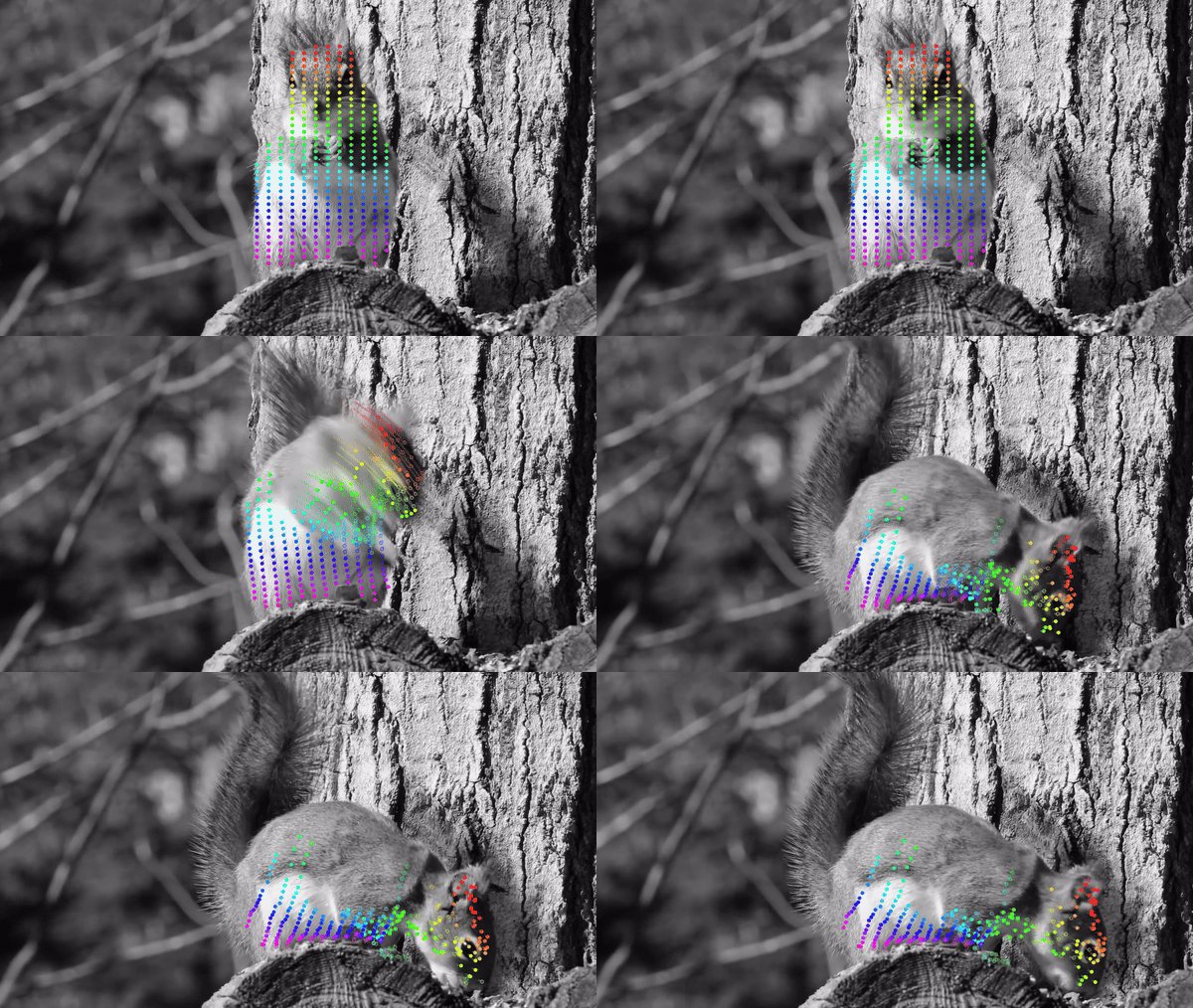
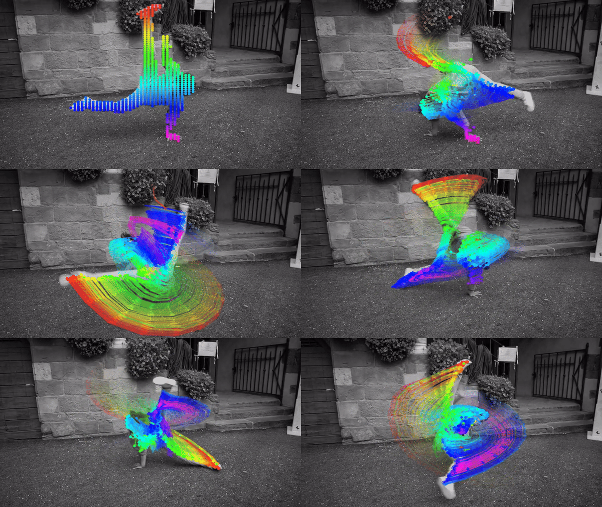
Traditionally, we use Optical Flow or Feature Tracking to track the pixels in motion video. However, optical flow only produces motion for adjacent frames, whereas feature tracking only tracks sparse pixels. So, what if we can track both the dense and long-range pixel trajectories in a video sequence? 

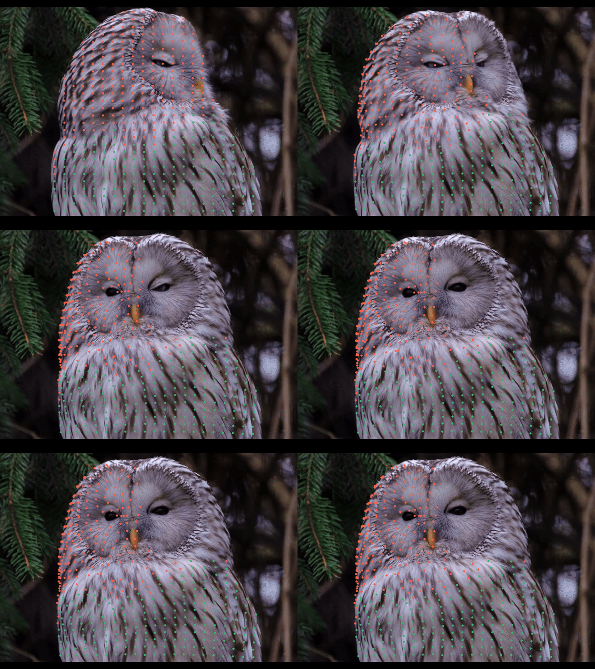
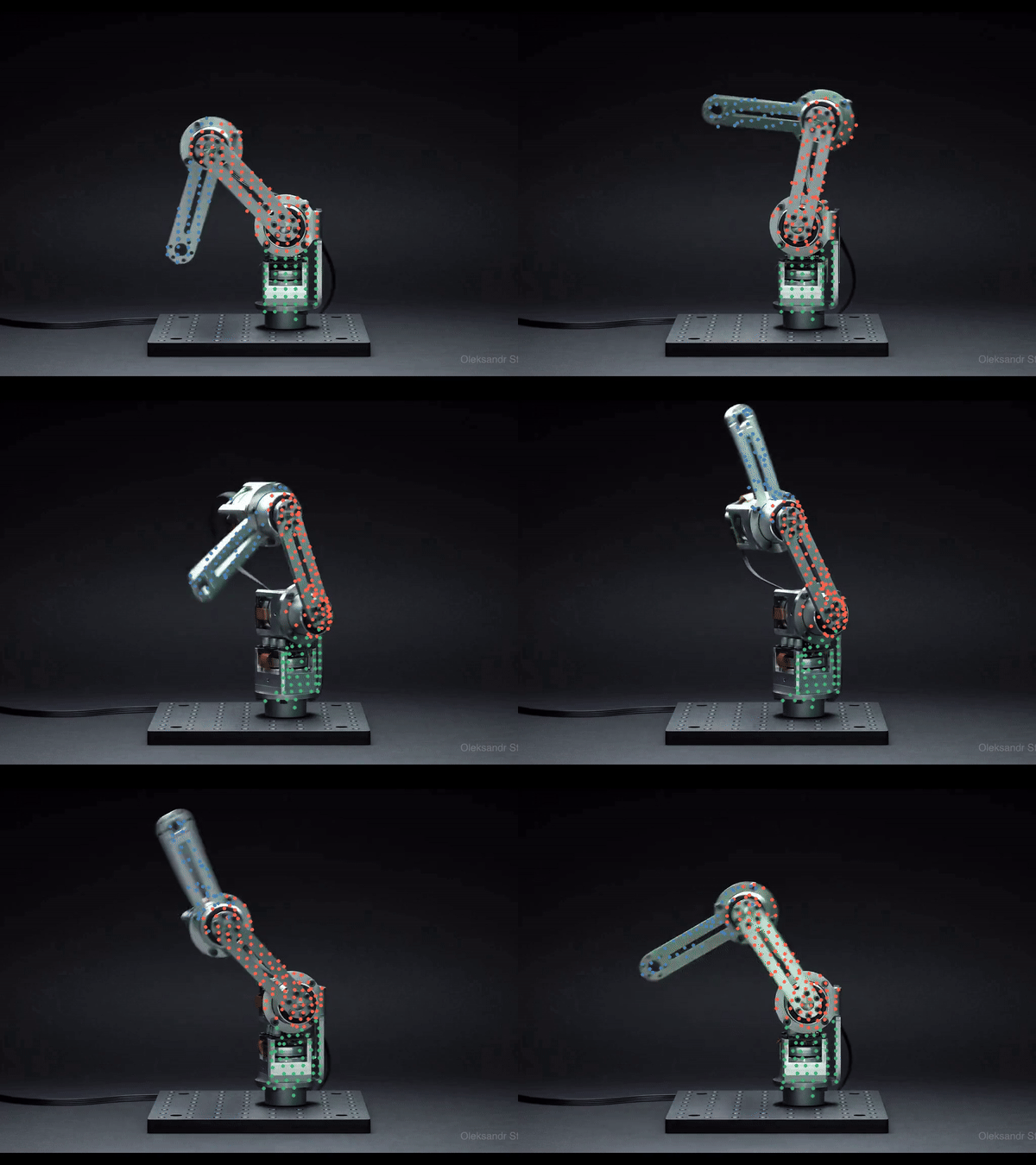
Yuxi Xiao, Qianqian Wang, et al. proposed SpatialTracker, which corresponds 2D pixels to 3D using monocular depth estimators, represents the 3D content of each frame efficiently using a triplane representation, and performs iterative updates using a transformer to estimate 3D trajectories. It takes the 3d space to track all the 2d pixels present in the video. Tracking in 3D allows us to leverage as-rigid-as-possible (ARAP) constraints while simultaneously learning a rigidity embedding that clusters pixels into different rigid parts. Using this method, authors were able to track long videos containing rigid or occluded parts without any issues.

Model Overview

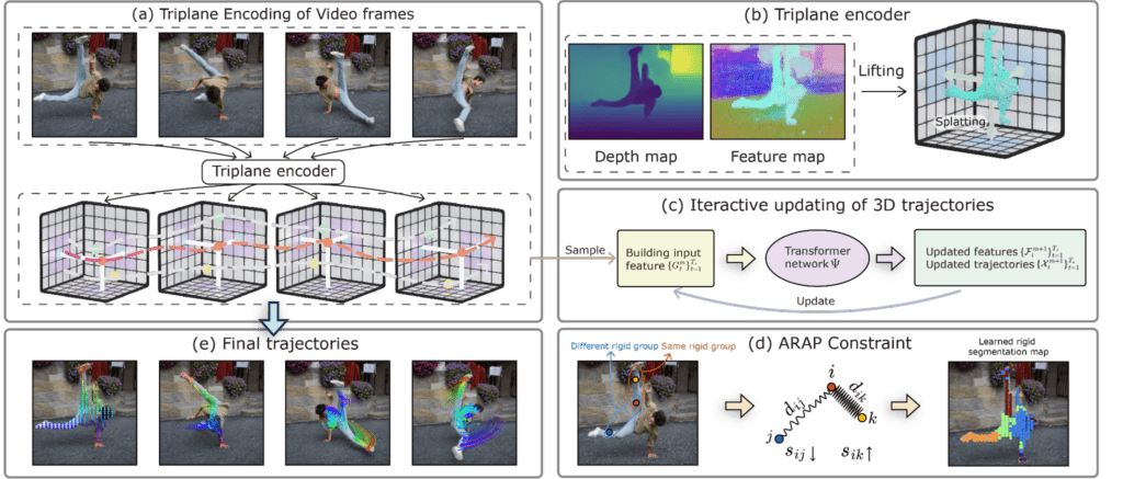
• First, using a triplane encoder, the model encodes each frame into a tri-plane representation.
• Then, it initializes and iteratively updates point trajectories in 3D space using a transformer that takes features extracted from these triplanes as input.
• These 3D point trajectories are trained with ground-truth annotations and regularized by an as-rigid-as-possible (ARAP) constraint with learned rigidity embedding.
• The ARAP constraint enforces that 3D distances between points with similar rigidity embeddings remain constant over time. Here, d_ij represents the distance between points i and j, while s_ij denotes the rigid similarity. This method produces accurate long-range motion tracks even under fast movements and severe occlusion.

More Examples

2D Tracking

Rigid Part Segmentation from Videos

Code Pipeline

The authors provided a GitHub repository, which is mentioned above. To run the code, you need to create a virtual env using:

conda create -n SpaTrack python==3.10

conda activate SpaTrack

Then, install the pytorch using:

pip install torch==2.1.1 torchvision==0.16.1 torchaudio==2.1.1 --index-url https://download.pytorch.org/whl/cu118

Then clone the repository using:

git clone https://github.com/henry123-boy/SpaTracker.git

Then, install the requirements:

pip install -r requirements.txt

Then, download and place the model checkpoints and dataset as mentioned in the GitHub readme.

And you are ready to go. Run the demo.py:

python demo.py --model spatracker --downsample 1 --vid_name sintel_bandage --len_track 1 --fps_vis 15  --fps 1 --grid_size 60 --gpu ${GPU_id} --point_size 1 --rgbd # --vis_support

All the flags are available in the GitHub repo itself.

Paper 7: ZeroNVS: Zero-Shot 360-Degree View Synthesis from a Single Real Image

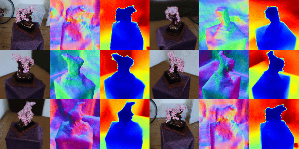
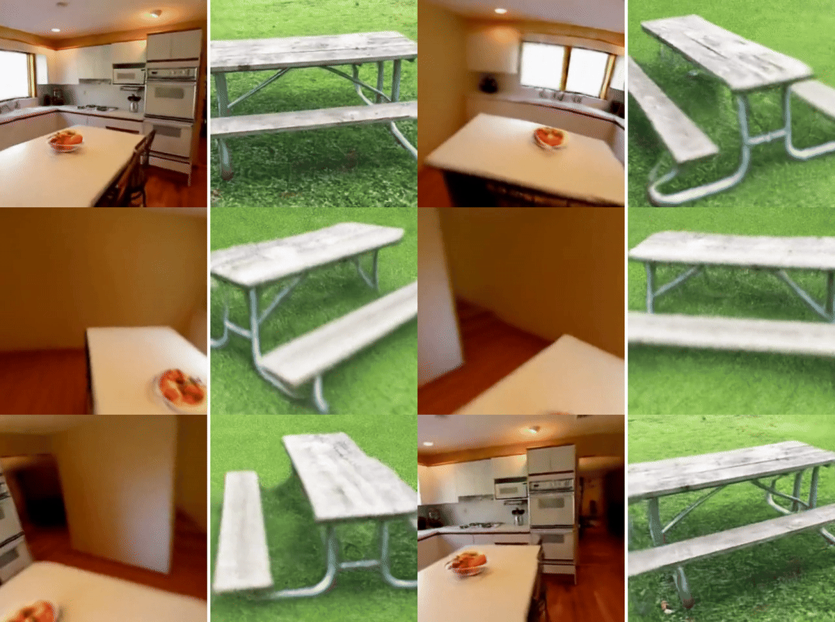
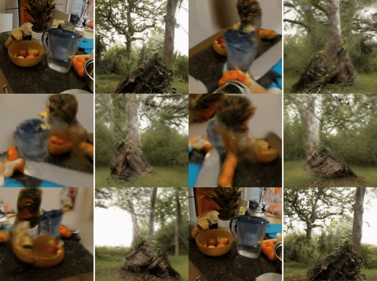
The paper by Kyle Sargent, Zizhang Li, et al. introduces ZeroNVS, a new 3d diffusion model designed to create 360-degree views from just a single image. It specifically tackles the tough challenge of handling scenes with multiple objects and complex backgrounds. Unlike traditional models focusing on simple scenes, ZeroNVS works with a mix of different scene types, from indoors to outdoors, helping it perform better in real-world settings. It uses a clever method called “SDS anchoring” to improve how diverse the backgrounds look in the generated views, which helps make the scenes look more realistic.

Method Overview

Representing Objects for View Synthesis:

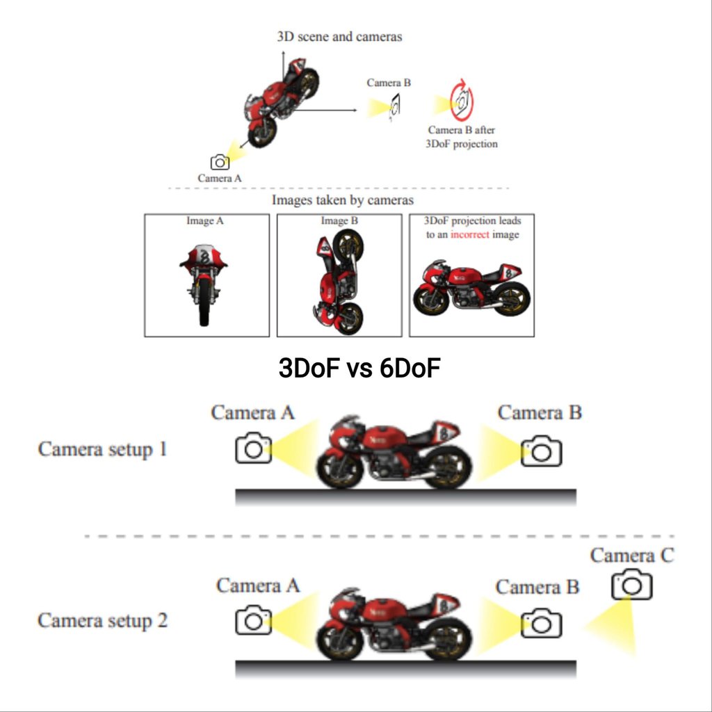
Traditionally, object poses in view synthesis are modeled using three degrees of freedom (3DoF), which include elevation, azimuth, and distance from the camera, suitable for simple, isolated objects. The innovation in ZeroNVS is its extension to six degrees of freedom (6DoF), capturing all rotational and translational movements, which allows it to accurately handle scenes with multiple, complex objects and varied orientations, thus providing a more realistic rendering of 3D scenes from single images.

Representing Scenes for View Synthesis:

Old-school models often drop the ball when they have to deal with complicated scenes. They just don’t get the full picture. ZeroNVS changes the game by being smart about how it thinks about camera settings, including how wide the camera lens is. This means it can capture all the tiny details and different perspectives that make a scene look just right, much like what you’d see with your own eyes.

Addressing Scale Ambiguity with a New Normalization Scheme:

Ever notice how, in photos, it’s hard to tell how big things are or how far away they are? ZeroNVS tackles this head-on. It uses information about how deep scenes go from several sources to figure out the right scale, ensuring everything looks the size it should. This is a big deal because it helps the model make sense of different scenes more reliably, keeping things looking real no matter where they’re from.

Improving Diversity with SDS Anchoring:

Conventional NVS techniques often produce limited background diversity, resulting in synthesized views that can appear monotonous or unrealistic. ZeroNVS tackles this problem with SDS anchoring, a technique that uses a preliminary sampling of diverse views via the DDIM sampling method. This technique starts with generating a set of diverse, preliminary views using DDIM sampling. These views are then used as reference points or ‘anchors’ to guide the diffusion process, thus ensuring that the backgrounds in the synthesized images are varied and more reflective of real-world variability.

More Examples

Code Walkthrough

First, clone the official repo:

git clone https://github.com/kylesargent/zeronvs.git

cd zeronvs

Create a virtual env and install all the required libraries:

conda create -n zeronvs python=3.8 pip
conda activate zeronvs

pip install torch==2.0.1+cu118 torchvision==0.15.2+cu118 --extra-index-url https://download.pytorch.org/whl/cu118

conda install -c "nvidia/label/cuda-11.8.0" cuda-toolkit

pip install ninja git+https://github.com/NVlabs/tiny-cuda-nn/#subdirectory=bindings/torch

pip install -r requirements-zeronvs.txt

pip install nerfacc -f https://nerfacc-bucket.s3.us-west-2.amazonaws.com/whl/torch-2.0.0_cu118.html

Finally, initialize and pull the code in the zeronvs_diffusion submodule.

cd zeronvs_diffusion
git submodule init
git submodule update
cd zero123
pip install -e .
cd ..
cd ..

Download and unzip the model and data:

gdown --fuzzy https://drive.google.com/file/d/1q0oMpp2Vy09-0LA-JXpo_ZoX2PH5j8oP/view?usp=sharing
gdown --fuzzy https://drive.google.com/file/d/1aTSmJa8Oo2qCc2Ce2kT90MHEA6UTSBKj/view?usp=drive_link
gdown --fuzzy https://drive.google.com/file/d/17WEMfs2HABJcdf4JmuIM3ti0uz37lSZg/view?usp=sharing
unzip dtu_dataset.zip

Finally, run the launch_inference.sh to run the inference on your own images.

CVPR 2024 – Special Mentions

As the article is already so long, it is not possible to cover all the papers in detail in this one. Maybe we will cover all the papers in detail in our future articles one by one, so keep an eye on LearnOpenCV. But we will not gonna leave you on a FOMO!

I will try adding a list of more interesting papers here for you. Go and check those out, too! 

DiffusionLight: Light Probes for Free by Painting a Chrome Ball

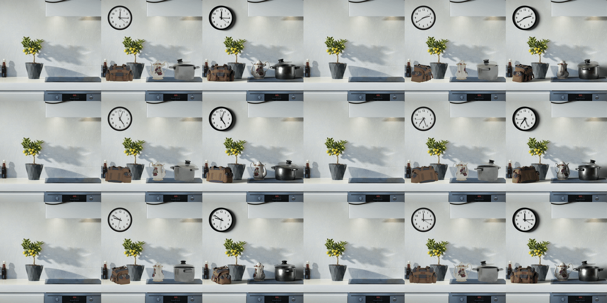
SpiderMatch: 3D Shape Matching with Global Optimality and Geometric Consistency

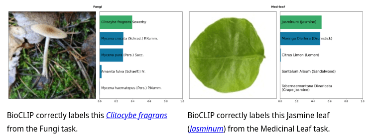
BioCLIP: A Vision Foundation Model for the Tree of Life

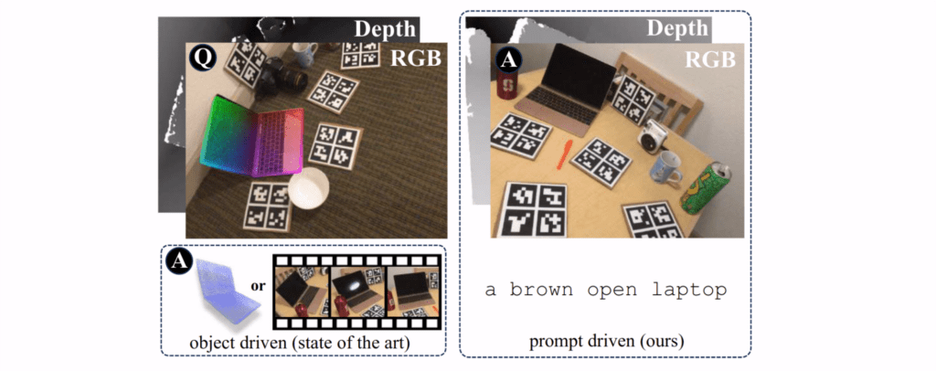
Oryon: Open-Vocabulary Object 6D Pose Estimation

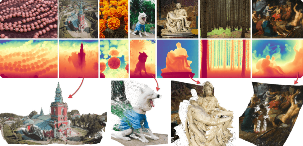
Repurposing Diffusion-Based Image Generators for Monocular Depth Estimation

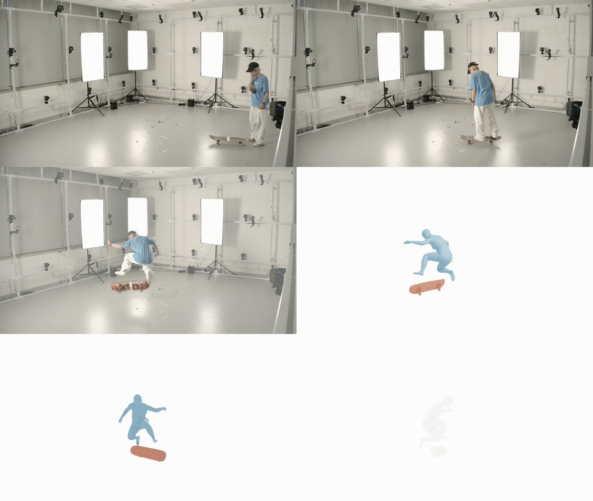
I’M HOI: Inertia-aware Monocular Capture of 3D Human-Object Interactions

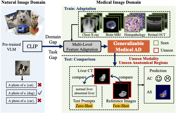
Adapting Visual-Language Models for Generalizable Anomaly Detection in Medical Images

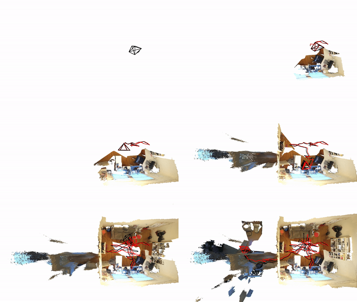
Loopy-SLAM: Dense Neural SLAM with Loop Closures

VideoSwap: Customized Video Subject Swapping with Interactive Semantic Point Correspondence

Conclusion

CVPR 2024 knocked it out of the park, offering a deep dive into the latest and greatest in AI and computer vision. We saw everything from creating dynamic videos to single images to cutting-edge video editing and 3D modeling techniques pushing the boundaries. This roundup touched on just a few standout papers, but the conference was packed with a lot more worth exploring.

In the second part of this article, we will cover a few more research papers and some good datasets. This year, 2719 papers were accepted out of 11532 submitted research papers. We tried our best to explore as much as we could. Let us know if you find any other good papers we have missed; we would love to include them, too!

References

Workbook: CVPR 2024

CVPR 2024 Paper Highlights

CVPR 2024 Best Paper Award Winners