The task of marking foreground entities plays an important role in the video pre-processing pipeline as the initial phase of computer vision (CV) applications. As examples of such applications, we can perform monitoring, tracking, and recognition of the objects: traffic analysis, people detection, tracking of the animals and others.

Steeping into the idea behind these CV-systems we can observe that in most cases the initial steps contain background subtraction (BS), which helps to obtain relatively rough and rapid identifications of the objects in the video stream for their further subtle handling. In the current post, we are going to cover several noteworthy algorithms in terms of accuracy and processing time BS methods: SuBSENSE and LSBP-based GSoC method.

The blog post is divided into the following sub-topics:

1. Basic concepts and approaches of Background Subtraction
2. Descriptors and Types
3. The SubSENSE Algorithm
   1. Implementation using BGS library
4. GSoC Algorithm
   1. Implementation using OpenCV library
5. Evaluation
6. Evaluation Pipeline
7. Results

Background Subtraction: Basic Concepts and Approaches

Background subtraction methods solve the task of the foreground extraction by creating a background model. The full BS pipeline may contain the following phases:

• background generation – processing N frames to provide the background image
• background modeling – defining the model for background representation
• background model update – introducing the model update algorithm for handling the changes, which occur over time
• foreground detection – dividing pixels into sets of background or foreground.

Background subtraction output consists of a binary mask, which separates frame pixels into two sets: foreground and background pixels.

It should be mentioned that frequently in the BS-approaches the focus is shifted to the implementation of the advanced background models and robust feature representation aspect.

Descriptors

Here we touched upon another important concept – descriptors (features). Descriptors define the captured image region in the current video frame for its mapping with a known background model. The goal of this comparison is to distinguish the region from the background or foreground. It can be done, for example, with color, texture and edge descriptors.

Obviously, BS-algorithm design, including a combination of the features, should be relied on the initial object field analysis. It’s needed to consider the possible challenging factors: specific illumination, oscillations, movement of objects and others.

For instance, suppose most of the background area is statical. Then it’s assumed that the color of the same regions is fixed, hence, we can identify the background. However, there are different foreground objects and illumination variations, which can distort the colors.

Types of Descriptors

Let’s examine the sorts of features and specific challenges for them. The pixel values of the frames are available during video processing. Thus, the computation of the pixel domain descriptors is widespread in the BS-algorithms. Popular pixel domain descriptors:

• color: descriptive object features. The components of the RGB color space are tightly connected, reacting to the illumination changes. There is no brightness and chroma separation (as in YCrCb). Color features are sensitive to the illumination, camouflage, shadows, which can affect the appearance of moving objects. That is the reason why usually they are combined with other features for more robustness.
• edge: edge features are robust to the light variations and good for the detection of the moving objects. Edge features are sensitive to both high and low textured objects.
• texture: texture features provide spatial information. They are robust to the illumination and shadows. For example, texture features are applied in the Local Binary Pattern (LBP).

Texture Features

In the current subchapter we will briefly overview the texture descriptors and their evolution.

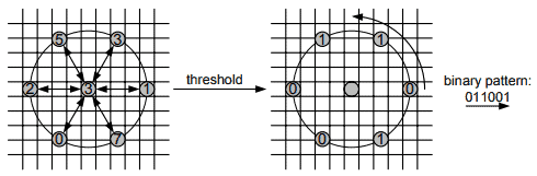
1. Local Binary Pattern (LBP). LBP was introduced in 2005 as “a gray-scale invariant texture primitive statistic” for texture description and defined the starting point for further development of texture descriptors. The LBP operator produces a binary pattern (number) labeling the frame pixels of the specified area by thresholding each neighboring pixel value with the value of the center pixel.



There are eight neighboring pixels in the basic LBP but the number can be extended. The drawback of the LBP is the absence of intensity tracking. The center pixel intensity value can stay more (or less) than neighboring values after scene change. Thus, the detection of changes can be failed.

2. Local Binary Similarity Patterns (LBSP). LBSP method was introduced in 2013 to solve the issue using absolute difference thresholding in comparison of the center and neighboring pixels. However, LBSP is not spatiotemporal, the information about features and intensity updates not simultaneously.

3. Self-balanced sensitivity segmenter (SuBSENSE). SuBSENSE was introduced in 2014. It uses improved spatiotemporal LBSP in combination with color features.
4. Background Subtraction using Local SVD Binary Pattern (LSBP). Local SVD Binary Pattern feature descriptor is robust to the illumination variations, shadows and noise. The coefficients of the singular value decomposition (SVD) used in LSBP characterize the illumination invariant.

In the following chapters we will explore SuBSENSE and GSoC methods in more detail.

SuBSENSE Algorithm

Overview

The below scheme presents the SuBSENSE functioning mechanism:

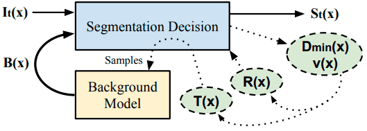
Suppose there is a video sequence as an input. Then is the result of the -th frame (at time ) spatial analysis, where is a pixel index. The background model block is a non-parametric statical model. It produces the background at pixel locations denoted by on the basis of 50 past representations (samples) . is a segmentation output. Its has the following values:

• : the pixel is marked as background, if there is an intersection of at least 2 samples with the representation of in the -th frame ()
• : the pixel is automatically marked as foreground in the opposite cases.

SuBSENSE solves the background subtraction problem as a classification task, where a pixel value is analyzed due to its neighboring pixels in the feature space. Hence, – modeling of pixel relying on the samples. These samples are randomly chosen at the background model initialization time. The SuBSENSE analysis core is color comparison and LBSP descriptors, calculated on the color channels. Thus, , where include the following: .

and are matched through the color values and LBSP-descriptors.

For the colors comparison L1 distance is used, whereas descriptors are compared with the Hamming distance. The resulting mask is binary and can be described as:

is the threshold of the maximum distance. Its value is dynamically assigned in accordance with the model loyalty, segmentation noise.

Implementation Using BGSLibrary

In the current subchapter we will experiment with background subtraction using BGS library API. It’s worth noting that the BGS framework was developed as a specialized OpenCV-based C++ project for video foreground-background separation. BGS library also has wrappers for Python, Java and MATLAB. Thus, BGS contains a wide range of background subtraction methods as it can be seen from its, for example, Python demo script.

As default input we will use a video sequence with a static background and dynamic foreground objects:

default="space_traffic.mp4"

Specify --input_video key to set another input video.

1. Video Processing

Upload and process video data with OpenCV VideoCapture:

# create VideoCapture object for further video processing
captured_video = cv2.VideoCapture(video_to_process)
# check video capture status
if not captured_video.isOpened:
    print("Unable to open: " + video_to_process)
    exit(0)

2. Model Initialization

Instantiate the model:

# instantiate background subtraction
background_subtr_method = bgs.SuBSENSE()

3. Obtaining results

Obtain the results (the initial size of frames was 1920×1080):

while True:
    # read video frames
    retval, frame = captured_video.read()

    # check whether the frames have been grabbed
    if not retval:
        break

    # resize video frames
    frame = cv2.resize(frame, (640, 360))

    # pass the frame to the background subtractor
    foreground_mask = background_subtr_method.apply(frame)
    # obtain the background without foreground mask
    img_bgmodel = background_subtr_method.getBackgroundModel()

4. Visualizing results

Visualize results with OpenCV imshow:

while True:
    # ...

    # show the current frame, foreground mask, subtracted result
    cv2.imshow("Initial Frames", frame)
    cv2.imshow("Foreground Masks", foreground_mask)
    cv2.imshow("Subtraction result", img_bgmodel)

    keyboard = cv2.waitKey(10)
    if keyboard == 27:
        break

The outputs are:

• initial frame:

• obtained foreground mask:

• subtraction result:

In the above case masks were detected more accurately, in general foreground objects were captured correctly, however, there are the following defects:

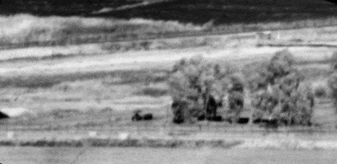
• statical group of people in the left part of the frame was not detected at all:

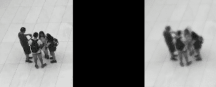
• almost statical objects with moving components:

• the regions, where people are close to each other were combined into one shared mask:

GSoC Algorithm

Overview

During Google Summer of Code (GSoC) 2017 the advancement of LSPB was provided: BackgroundSubtractorGSOC. GSoC BS-method was introduced in order to make LSBP faster and more robust. The method relies on RGB color values instead of LSBP descriptors and achieves high performance on the CDnet-2012.

GSoC BS-implementation doesn`t refer to any article, therefore let’s view the basic points by exploring its source bgfg_gsoc.cpp. Firstly, we need to pay attention to the BackgroundSubtractorGSOC instantiation parameters:

Ptr< BackgroundSubtractorGSOC > createBackgroundSubtractorGSOC(
     int mc,
     int nSamples,
     float replaceRate,
     float propagationRate,
     int hitsThreshold,
     float alpha,
     float beta,
     float blinkingSupressionDecay,
     float blinkingSupressionMultiplier,
     float noiseRemovalThresholdFacBG,
     float noiseRemovalThresholdFacFG
)

There are the following meanings behind them:

• mc: camera motion compensation flag
• nSamples: number of samples to maintain at each point of the frame.
• replaceRate: probability of replacing the old sample – how fast the model will be updated.
• propagationRate: probability of propagating to neighbors.
• hitsThreshold: how many positives the sample must get before it will be considered as a possible replacement.
• alpha: scale coefficient for threshold.
• beta: bias coefficient for threshold.
• blinkingSupressionDecay: blinking suppression decay factor.
• blinkingSupressionMultiplier: blinking suppression multiplier.
• noiseRemovalThresholdFacBG: strength of the noise removal for background.
• noiseRemovalThresholdFacFG: strength of the noise removal for foreground .

Keeping the above data in mind let’s examine the core BS-part described in apply() method. The computation core init is in apply():

parallel_for_(Range(0, sz.area()), ParallelGSOC(sz, this, frame, learningRate, fgMask));

The ParallelGSOC contains comparison operations of the neighboring pixels relying on RGB color features.

Another important point concerns the type of frame pixels. The pixels, which frequently switch between the foreground and background are defined as blinking. GSoC BS-approach applies a special heuristic for blinking pixels detection:

cv::add(blinkingSupression, (fgMask != prevFgMask) / 255, blinkingSupression, cv::noArray(), CV_32F);
blinkingSupression *= blinkingSupressionDecay;
fgMask.copyTo(prevFgMask);
Mat prob = blinkingSupression * (blinkingSupressionMultiplier * (1 - blinkingSupressionDecay) / blinkingSupressionDecay);

for (int i = 0; i < sz.height; ++i)
    for (int j = 0; j < sz.width; ++j)
        if (rng.uniform(0.0f, 1.0f) < prob.at< float >(i, j))
            backgroundModel->replaceOldest(i, j, BackgroundSampleGSOC(frame.at< Point3f >(i, j), 0, currentTime));

Here the blinkingSupression can be defined as a blinking pixel map obtained by current and previous mask XOR. Then the values obtained with blinking suppression coefficients are picked at random for classifying of the appropriate pixels as background.

Produced mask postprocessing step is final and consists of denoising and gaussian blur:

void BackgroundSubtractorGSOCImpl::postprocessing(Mat& fgMask) {
    removeNoise(fgMask, fgMask, size_t(noiseRemovalThresholdFacBG * fgMask.size().area()), 0);
    Mat invFgMask = 255 - fgMask;
    removeNoise(fgMask, invFgMask, size_t(noiseRemovalThresholdFacFG * fgMask.size().area()), 255);

    GaussianBlur(fgMask, fgMask, Size(5, 5), 0);
    fgMask = fgMask > 127;
}

The threshold value for the noise removal is produced with noiseRemovalThresholdFacBG and noiseRemovalThresholdFacBG multiplication on the mask area. Further the mask values are updated in accordance with the obtained threshold:

for (int i = 0; i < sz.height; ++i)
    for (int j = 0; j < sz.width; ++j)
        if (compArea[labels.at< int >(i, j)] < threshold)
            fgMask.at< uchar >(i, j) = filler;

Implementation Using OpenCV

In the current section we will experiment with background subtraction using the appropriate API from the OpenCV library by the example of default "space_traffic.mp4" video.

1. Video Processing

Upload and process video data with OpenCV VideoCapture:

# create VideoCapture object for further video processing
captured_video = cv2.VideoCapture(video_to_process)
# check video capture status
if not captured_video.isOpened:
    print("Unable to open: " + video_to_process)
    exit(0)

2. Model Initialization

Instantiate the model:

# instantiate background subtraction
background_subtr_method = cv2.bgsegm.createBackgroundSubtractorGSOC()

3. Obtaining results

Obtain the results (the initial size of frames was 1920×1080):

while True:
    # read video frames
    retval, frame = captured_video.read()

    # check whether the frames have been grabbed
    if not retval:
        break

    # resize video frames
    frame = cv2.resize(frame, (640, 360))

    # pass the frame to the background subtractor
    foreground_mask = background_subtr_method.apply(frame)
    # obtain the background without foreground mask
    background_img = background_subtr_method.getBackgroundImage()

4. Visualizing results

Visualize results with OpenCV imshow:

while True:
    # ...

    # show the current frame, foreground mask, subtracted result
    cv2.imshow("Initial Frames", frame)
    cv2.imshow("Foreground Masks", foreground_mask)
    cv2.imshow("Subtraction Result", background_img)

    keyboard = cv2.waitKey(10)
    if keyboard == 27:
        break

The outputs are:

• initial frame:

• obtained foreground mask:

• subtraction result:

We can see that mostly foreground objects were correctly located. However, there are some artifacts:

• masks of the foreground cover some extra space at the footing of the objects, which denotes their shadows:

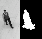
• statical objects were partially defined, only their moving components were detected, for example, moving man’s hand in the below picture:

  

  or some parts of the non-dynamic people group in the left part of the frame:

It can be noted that the most challenging areas for both algorithms contain statical foreground objects or partly moving objects with some dynamic components.

Evaluation

Data Sets

In the current post, we will use two datasets from ChangeDetection.NET(CDNET): CDNET-2012 and CDNET-2014 to provide an evaluation of the proposed BS-methods. CDNET data set is frequently used video collection for evaluation of algorithms due to the variety of its content: categories, input frames and corresponding ground truth (GT) images. There are 6 categories in CDNET-2012 and 11 in CDNET-2014. Let’s quickly look through them and view the video fragments:

Common categories:

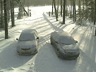
1. baseline: 4 videos with a statical background containing moving foreground objects

2. cameraJitter: 4 videos with slight camera oscillation effect

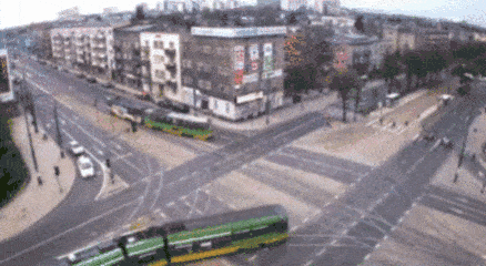
3. dynamicBackground: 6 videos with partly moving background and dynamic foreground

4. intermittentObjectMotion: 6 videos containing statical background with periodic moving foreground entities

5. shadow: 6 video sequences, which contain the shadows of the foreground objects

6. thermal: 5 videos obtained from a thermal camera

Introduced in CDNET-2014:

7. badWeather: 4 videos of traffic with poor visibility, distorted by snowfall images

8. lowFramerate: 4 video sequences with the low frame rate

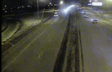
9. nightVideos: 6 videos containing low illuminated views

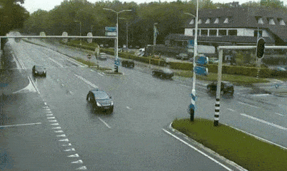
10. PTZ: 4 video sequences obtained with a pan-tilt-zoom camera (dynamic foreground: rotation, zoom; slight oscillation effect)

11. turbulence: 4 videos distorted with a slight ripple.

Evaluation Pipeline

To evaluate the algorithms we will use evaluator.py, based on opencv-contrib evaluation pipeline. To run the script we need to obtain the data set, in our case CDnet-2012 and CDnet-2014. The path to the data should be specified in --dataset_path required parameter. The below line initiates evaluation execution:

python evaluator.py --dataset_path ./cdnet_12

In the below lines we define the list of algorithms to evaluate (method creator, its title, passing arguments):

import cv2
import pybgs as bgs

ALGORITHMS_TO_EVALUATE = [
    (cv2.bgsegm.createBackgroundSubtractorGSOC, "GSoC", {}),
    (bgs.SuBSENSE, "SuBSENSE", {}),
]

Iterating over ALGORITHMS_TO_EVALUATE the specified background subtraction models are instantiated. To compute a foreground mask the apply(frame) method should be called. The mask list accumulates obtained foreground masks for further calculation of the algorithm quality metrics. Before we get their values, let’s remember the following key concepts:

• true positives () – properly masked objects
• true negatives () – properly not masked objects
• false positives () – improperly masked objects
• false negatives () – improperly not masked objects. Knowing , , and values we can calculate precision, recall and, finally, -measure and accuracy value:
  1. precision – the ratio of true positives in the obtained results:
  2. recall – the amount of true positives found among all the ground truth:
  1. F1-measure (FM):
  2. Accuracy:

Results

The minimal F1 value 0.084 for LSBP was obtained in dynamicBackground video series:

	Precision	Recall	F1	Accuracy
LSBP:	0.064	0.784	0.084	0.864
GSoC:	0.269	0.913	0.289	0.990
SuBSENSE:	0.610	0.740	0.528	0.996

The most challenging videos for GSoC were from PTZ category:

	Precision	Recall	F1	Accuracy
LSBP:	0.231	0.639	0.216	0.888
GSoC:	0.246	0.933	0.265	0.811
SuBSENSE:	0.527	0.730	0.485	0.964

SuBSENSE showed the lowest F1 in nightVideos:

	Precision	Recall	F1	Accuracy
LSBP:	0.467	0.392	0.296	0.977
GSoC:	0.294	0.780	0.342	0.947
SuBSENSE:	0.462	0.624	0.448	0.975

The average values for all categories presented in the data sets are:

• CDnet-2012:

	Precision	Recall	F1	Accuracy
LSBP	0.491	0.643	0,393	0.93
GSoC	0,705	0,714	0,562	0,972
SuBSENSE	0,824	0,742	0,688	0,982

• CDnet-2014:

	Precision	Recall	F1	Accuracy
LSBP	0.455	0.624	0.362	0.945
GSoC	0.610	0.753	0.522	0.960
SuBSENSE	0.747	0.734	0.644	0,983

The above evaluations illustrate that in OpenCV category GSoC BS-method exceeds the LSBP values. SuBSENSE outperforms all the methods.

References

The following links contain detailed information about the above methods and additional materials for further exploration:

1. On the Role and the Importance of Features for Background Modeling and Foreground Detection: contains basic information about BS and its methods, detailed information about types of features, helpful illustrative comparative tables
2. Background Subtraction using Local SVD Binary Pattern: describes the LSBP method
3. Flexible Background Subtraction With Self-Balanced Local Sensitivity: describes SuBSENSE method
4. Regularly updating compilation of BS materials
5. CDnet datasets

Subscribe & Download Code

If you liked this article and would like to download code (C++ and Python) and example images used in this post, please subscribe to our newsletter. You will also receive a free Computer Vision Resource Guide. In our newsletter, we share OpenCV tutorials and examples written in C++/Python, and Computer Vision and Machine Learning algorithms and news.