U2-Net (popularly known as U2-Net) is a simple yet powerful deep-learning-based semantic segmentation model that revolutionizes background removal in image segmentation. Its effective and straightforward approach is crucial for applications where isolating foregrounds from backgrounds is beneficial and essential. This capability has significant implications for fields such as advertising, filmmaking, and medical imaging.
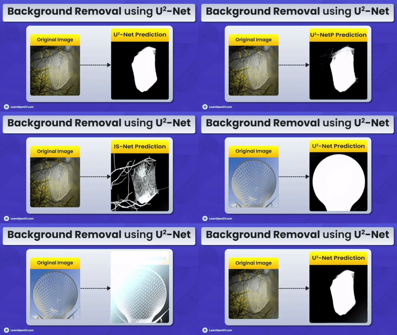
This article is aimed at intermediate to advanced readers interested in mastering background subtraction using image segmentation. U2-Net stands out by focusing on binary segmentation, offering a clear advantage over traditional semantic segmentation models. Given the limited high-quality content on this topic, our goal is to provide valuable insights into using U2-Net for efficient background removal.
We will also discuss IS-Net, an enhanced version of U2-Net, showcasing its superior results. This article will present impressive outcomes on challenging images, demonstrating the model’s capability. We hope to show that precise background removal is achievable and encourage readers to apply these models to their projects.
By the end of this article, you’ll understand why background removal is a complex yet vital task and how U2-Net and IS-Net are making significant strides in this area.
Scroll through the stunning inference results from U2-Net and IS-Net for a quick look.
- Why U2-Net for Foreground Estimation?
- Architecture of ReSidual U-block (RSU) in the Context of U2-Net
- U2-Net Architecture Explanation
- Training and Evaluation Strategies for U2-Net
- Qualitative Analysis of U2-Net Predictions
- IS-Net Architecture: Advancing U2-Net for Image Segmentation
- Inference Results from IS-Net
- Key Takeaways
- Conclusion
- References
Why U2-Net for Foreground Estimation?
Deep learning segmentation architectures, such as Fully Convolutional Networks (FCNs), tend to capture more semantic information through local feature extraction as we go deeper through the network with reduced feature map resolutions (as a consequence of multiple pooling operations). However, they miss the global contextual information extracted from the feature maps across multiple scales.
Newer approaches, such as DeepLab, mitigate information loss across multiple scales by increasing the network’s receptive field through multiple dilated convolutions (also known as atrous convolutions). However, this incurs significant computation costs during training with higher image resolutions.
The authors propose the U2-Net architecture that can handle both multi-level deep feature extraction and multi-scale information across local and global contexts. This two-level nested modified U-Net-like structure enables training without significant memory consumption and computation costs. The core of each level in the architecture is built upon the ReSidual U-block (RSU), which incorporates the properties of a residual block and a U-Net-like symmetric encoder-decoder structure.
Moreover, the U2-Net architecture performs better without using pre-trained classification backbones, enabling it to be trained from scratch.
In the next section, we will explore the RSU block in more detail.
Architecture of ReSidual U-block (RSU) in the Context of U2-Net
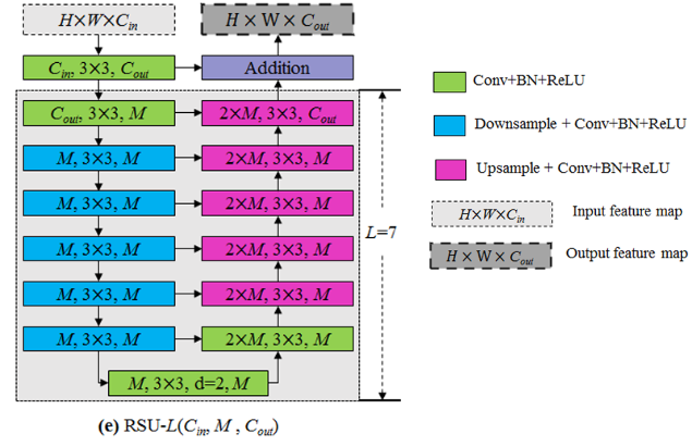
An RSU-L (L being the number of layers in the encoder) block can be structurally represented as RSU-L(Cin, M, Cout), where:
- Cin is the channel of the input feature map
- M is the number of channels for the intermediate layers in the encoder
- Cout is the channel for the output feature map.
Note that the spatial resolution of the output feature map from any RSU-L block remains identical to that of the input feature map.
A concise representation of an RSU-7 block is provided in the paper, as shown below.
Source U2 Net Going Deeper with Nested U Structure for Salient Object Detection
The Residual-U blocks primarily comprise the three components:
- An input convolution layer that transforms an input feature map (of shape:
[HxWxCin]) to an intermediate feature map of shape
 HxWxCoutto learn the local features.
- A U-Net-like symmetric encoder-decoder block that takes the feature map
 and learns to encode the multi-scale features
  . These multi-scale features are then extracted from the downsampled feature maps from the encoder layers through subsequent concatenation, convolution, and upsampling (in that order). The resolution from the final feature map
  is again
 HxWxCout.
The downsampling occurs due to the pooling operation, while a “bilinear” upsampling is used in the decoding phase. - A residual connection to fuse the local and multi-scale features through addition:
 .
.
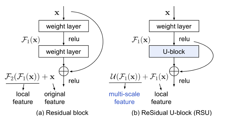
The RSU block is analogous to a residual block where we can learn multi-scale features instead of a convolution block to learn local features.
Source U2 Net Going Deeper with Nested U Structure for Salient Object Detection
In the diagram above, ![]() and
and ![]() are the feature representations learned from the weight (convolution) layers, and
are the feature representations learned from the weight (convolution) layers, and ![]() are the multi-scale features learned from encoder-decoder blocks.
are the multi-scale features learned from encoder-decoder blocks.
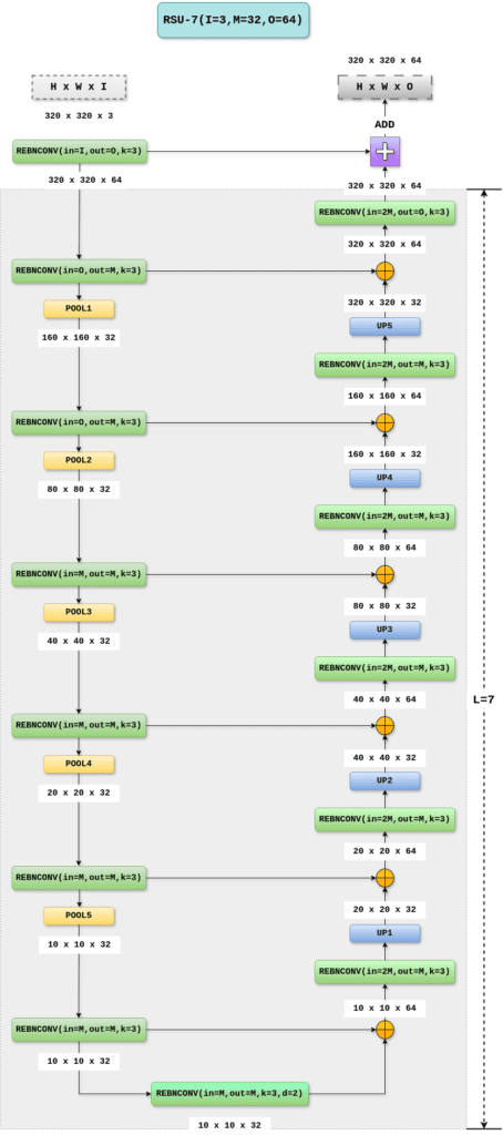
We will now present a more detailed block diagram for RSU-7, which has an input feature map with a resolution of 320x320x3. The notations I, M, and O represent the number of input, intermediate, and final output channels in the RSU block, respectively. The diagram also ascertains the shapes resulting from convolution, pooling, concatenation, and upsampling.
The REBNCONV block is the usual convolution followed by Batch Norm and ReLU activation (in that order).
The default padding and dilation rate is 1*d, where d assumes a default value of 1. So, if d is set to 2, then both padding and dilation rate are set to 2.
The ⊕ symbol in the diagram below refers to the concatenation operation.
320x320x3Code Explanation for RSU block
To better understand the implementation of the RSU7 module, let’s first review the REBNCONV module and its _upsample_like helper function:
1. The REBNCONV block applies the convolution followed by Batch Norm and ReLU to an intermediate feature map (as discussed in the previous diagram).
class REBNCONV(nn.Module):
    def __init__(self,in_ch=3,out_ch=3,dirate=1):
        super(REBNCONV,self).__init__()

        self.conv_s1 = nn.Conv2d(in_ch,out_ch,3,padding=1*dirate,dilation=1*dirate)
        self.bn_s1 = nn.BatchNorm2d(out_ch)
        self.relu_s1 = nn.ReLU(inplace=True)

    def forward(self,x):

        hx = x
        xout = self.relu_s1(self.bn_s1(self.conv_s1(hx)))

        return xout
2. The function _upsample_like accepts feature maps src and tar and subsequently upsamples src to have the sample spatial resolution of tar.
def _upsample_like(src,tar):

    src = F.upsample(src,size=tar.shape[2:],mode='bilinear')

    return src
We will begin by analyzing the RSU7 Module’s __init__ method for initializing the encoder, decoder, and pooling layers.
class RSU7(nn.Module):#UNet07DRES(nn.Module):

    def __init__(self, in_ch=3, mid_ch=12, out_ch=3):
        super(RSU7,self).__init__()

        self.rebnconvin = REBNCONV(in_ch,out_ch,dirate=1)

        self.rebnconv1 = REBNCONV(out_ch,mid_ch,dirate=1)
        self.pool1 = nn.MaxPool2d(2,stride=2,ceil_mode=True)

        self.rebnconv2 = REBNCONV(mid_ch,mid_ch,dirate=1)
        self.pool2 = nn.MaxPool2d(2,stride=2,ceil_mode=True)

        self.rebnconv3 = REBNCONV(mid_ch,mid_ch,dirate=1)
        self.pool3 = nn.MaxPool2d(2,stride=2,ceil_mode=True)

        self.rebnconv4 = REBNCONV(mid_ch,mid_ch,dirate=1)
        self.pool4 = nn.MaxPool2d(2,stride=2,ceil_mode=True)

        self.rebnconv5 = REBNCONV(mid_ch,mid_ch,dirate=1)
        self.pool5 = nn.MaxPool2d(2,stride=2,ceil_mode=True)

        self.rebnconv6 = REBNCONV(mid_ch,mid_ch,dirate=1)

        self.rebnconv7 = REBNCONV(mid_ch,mid_ch,dirate=2)

        self.rebnconv6d = REBNCONV(mid_ch*2,mid_ch,dirate=1)
        self.rebnconv5d = REBNCONV(mid_ch*2,mid_ch,dirate=1)
        self.rebnconv4d = REBNCONV(mid_ch*2,mid_ch,dirate=1)
        self.rebnconv3d = REBNCONV(mid_ch*2,mid_ch,dirate=1)
        self.rebnconv2d = REBNCONV(mid_ch*2,mid_ch,dirate=1)
        self.rebnconv1d = REBNCONV(mid_ch*2,out_ch,dirate=1)
- The
rebnconvinblock acts as an additional layer outside the encoder-decoder blocks, transforming the input feature map to pass through the subsequent encoder-decoder blocks. Interestingly, the feature map output from this layer is finally added to the final decoder output.
- Attributes
rebnconv1throughrebnconv7represent the encoder blocks, while the max-pooling layerspool1throughpool5are used for downsampling the features maps from encoder blocksrebnconv1throughrebnconv5, respectively.
- Attributes
rebnconv6dthroughrebnconv1drepresent the decoder blocks that extract the multi-scale features from the subsequent encoder layersrebnconv7throughrebnconv1in a bottom-up fashion.
Lastly, we will discuss the forward step for the RSU7 module:
    def forward(self,x):

        hx = x
        hxin = self.rebnconvin(hx)

        hx1 = self.rebnconv1(hxin)
        hx = self.pool1(hx1)

        hx2 = self.rebnconv2(hx)
        hx = self.pool2(hx2)

        hx3 = self.rebnconv3(hx)
        hx = self.pool3(hx3)

        hx4 = self.rebnconv4(hx)
        hx = self.pool4(hx4)

        hx5 = self.rebnconv5(hx)
        hx = self.pool5(hx5)

        hx6 = self.rebnconv6(hx)

        hx7 = self.rebnconv7(hx6)

        hx6d =  self.rebnconv6d(torch.cat((hx7,hx6),1))
        hx6dup = _upsample_like(hx6d,hx5)

        hx5d =  self.rebnconv5d(torch.cat((hx6dup,hx5),1))
        hx5dup = _upsample_like(hx5d,hx4)

        hx4d = self.rebnconv4d(torch.cat((hx5dup,hx4),1))
        hx4dup = _upsample_like(hx4d,hx3)

        hx3d = self.rebnconv3d(torch.cat((hx4dup,hx3),1))
        hx3dup = _upsample_like(hx3d,hx2)

        hx2d = self.rebnconv2d(torch.cat((hx3dup,hx2),1))
        hx2dup = _upsample_like(hx2d,hx1)

        hx1d = self.rebnconv1d(torch.cat((hx2dup,hx1),1))

        return hx1d + hxin
Figure 3. illustrates how convolution, downsampling, concatenation, and upsampling are done across the multiple encoder-decoder blocks.
Observe that the final addition happens from the outputs of the rebnconvin and the `rebnconv1d` decoder layers.
Prior to explaining the U2-Net architecture, please note that the authors also use a modified version of the RSU block that replaces the pooling and upsampling layers in the encoder-decoder blocks with dilated convolutions. This is done to mitigate the gradual loss of contextual information across the deeper stages in the network. This block is called the RSU-KF block, where K is the number of layers in the encoder.
U2-Net Architecture Explanation
The core of the U2-Net architecture is the residual-U (RSU) block described in the previous section. The “squared” exponentiation comes from the network built on a two-level nested structure. The outer level maintains a U-structure composed of 11 stages, each comprising a configured RSU block.
The block diagram is shown below.
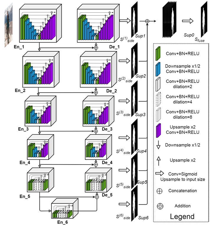
Source U2 Net Going Deeper with Nested U Structure for Salient Object Detection
The U2-Net structure consists of the following three components:
- The six encoder stages: En_1, En_2, En_3, En_4, En_5, and En_6. Stages 1-4 follow the RSU-7, RSU-6, RSU-5, and RSU-4 blocks; while stages 5 and 6 implements the RSU-4F block mentioned earlier.
- The five decoder stages, De_1, De_2, De_3, De_4, and De_5, follow similar RSU architectures as their symmetric encoder counterparts. Each decoder (except De_5, which takes the upsampled concatenation of output feature maps from En_5 and En_6) takes the upsampled concatenation of the output from its previous stage and its symmetric encoder stage.
- The feature map outputs from the decoder stages De_1 to De_5 and the encoder stage En_6 are then convolved using a 3×3 convolution layer and upsampled to the input image resolution (
320x320) to produce six-side feature outputs: , and
, and  , which are then activated using the sigmoid activation function to produce the output probability maps.
These feature outputs are concatenated, followed by a1x1convolution and the sigmoid activation to produce the final probability map .
.
The table below shows the complete configuration parameters of the RSU blocks across U2-Net’s encoder and decoder stages.

Although the complete U2-Net architecture is built using the RSU blocks, the implementation details for the final layers of the architecture are worth mentioning since we will use them during inference.
Let us now focus on the final side outputs implemented at the U2NET module’s forward step.
        #side output
        d1 = self.side1(hx1d)

        d2 = self.side2(hx2d)
        d2 = _upsample_like(d2,d1)

        d3 = self.side3(hx3d)
        d3 = _upsample_like(d3,d1)

        d4 = self.side4(hx4d)
        d4 = _upsample_like(d4,d1)

        d5 = self.side5(hx5d)
        d5 = _upsample_like(d5,d1)

        d6 = self.side6(hx6)
        d6 = _upsample_like(d6,d1)

        d0 = self.outconv(torch.cat((d1,d2,d3,d4,d5,d6),1))

        return F.sigmoid(d0), F.sigmoid(d1), F.sigmoid(d2), F.sigmoid(d3), F.sigmoid(d4), F.sigmoid(d5), F.sigmoid(d6)
Attributes side1 through side6 are the 3x3 convolutions applied to the output features from the decoder stages hx1d through hx5d (De_1 to De_5) and the encoder stage hx6. The upsampled side outputs are concatenated and passed through a 1x1 convolution (outconv). Finally, the sigmoid activation is applied to all the individuals and the concatenated side outputs.
The authors also provide a smaller version of the U2–Net model called U2-NetP targeted for edge-device inference. It consists of the reduced number of the input, intermediate, and output channels in the RSU blocks.
Did you know that background subtraction can also be used for document alignment? Our Automated Document Alignment article describes how we fine-tune DeepLabv3 to segment and align documents automatically.
Training and Evaluation Strategies for U2-Net
Now that we have an in-depth understanding of the U2-Net architecture, we will also discuss the various strategies the authors have employed to train the U2-Net model.
Training Dataset and Augmentation
The authors used the DUTS Image dataset for this binary segmentation. The training data contains 10553 images, further augmented through horizontal flipping to obtain 21106 training images offline.
During training, the images are first resized to 320×320 resolution, then randomly vertically flipped, and finally randomly cropped to 228×288 resolution.
Loss and Optimizer for U2-Net Training
The training loss is defined as the weighted sum of the losses from the side output probability maps and that of the final fused (concatenated) output map.

M is set to 6, indicating the six-side output saliency maps. The side and the fused weights (![]() and
and ![]() ) are set to 1. Each loss term, l, is the standard Binary Cross-Entropy loss:
) are set to 1. Each loss term, l, is the standard Binary Cross-Entropy loss:
![$$l = - \sum_{(r,c)}^{(H,W)} {[P_{G(r,c)}\log P_{S(r,c)} + (1-P_{G(r,c)})\log (1-P_{S(r,c)})}]$$](https://learnopencv.com/wp-content/ql-cache/quicklatex.com-da41a876eb130c27d076e92d27d72417_l3.png)
Where (r,c) indicates the pixel location and H and W represent the image height and width, respectively. ![]() and
and ![]() refer to the ground truth and the predicted probability pixel values, respectively.
refer to the ground truth and the predicted probability pixel values, respectively.
The authors used Adam optimizer to train the network with the default hyperparameters with an initial learning rate of 1e-3, betas=(0.9, 0.999), eps=1e-8, and weightdecay=0.
Evaluation Datasets and Metrics
Six benchmark datasets were used for evaluation: DUT-OMRON (5168 images), DUTS-TE (5019 images), HKU-IS (4447 images), ECSSD (1000 images), PASCAL-S (850 images), SOD (300 images).
The following evaluation metrics were used to report the performance of the U2-Net model:
- Precision-Recall Curve
- The beta-F-score measure (higher the better) is given as follows:

- Mean absolute Error (MAE – lower the better) between the ground truth mask and the predicted map; given as:

- Weighted F-score (higher the better) to overcome the possible unfair comparison caused by “interpolation flaw, dependency f law and equal-importance flaw”; given as:

- S-measure (Sm – higher the better) is used to evaluate the structure similarity of the predicted non-binary saliency map and the ground truth. The S-measure is defined as the weighted sum of region-aware Sr and object-aware So structural similarity:

- The relax boundary F-measure (
 —higher the better) is used to quantitatively estimate the predicted mask’s boundary quality.
The following table shows the metric scores across the six datasets used during the evaluation.

U^2-Net achieves almost state-of-the-art results on the DUT-OMRON, the HKU-IS, and the ECSSD datasets, as vindicated by the scores highlighted in red (scores in green and blue indicate the second and the third best scores). It almost achieves the second-best performance on the DUTS-TE and the SOD data. Even though the performance of U2-Net on the PASCAL-S data is inferior, the scores are almost closer to the top 3 scores.
Qualitative Analysis of U2-Net Predictions
Next, let’s perform the inference on some sample images. We shall visualize the results using both easy and challenging examples.
We will use both UNet and UNetP models for inference. The script u2net.py contains the model architecture definition, supporting modules, and helper functions.
We will start with our imports.
import os
from PIL import Image
import numpy as np

from torchinfo import summary

import torch
import torchvision.transforms as T

from u2net import U2NET, U2NETP

import torchvision.transforms.functional as F
Loading U2-Net and U2-NetP Weights
First, we will initialize the U2NET and U2NETP models.
u2net = U2NET(in_ch=3,out_ch=1)
u2netp = U2NETP(in_ch=3,out_ch=1)
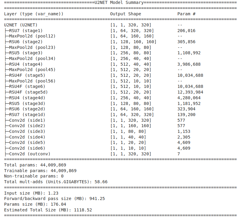
The figure below shows the model summary for U2NET. The model has approximately 44M parameters.
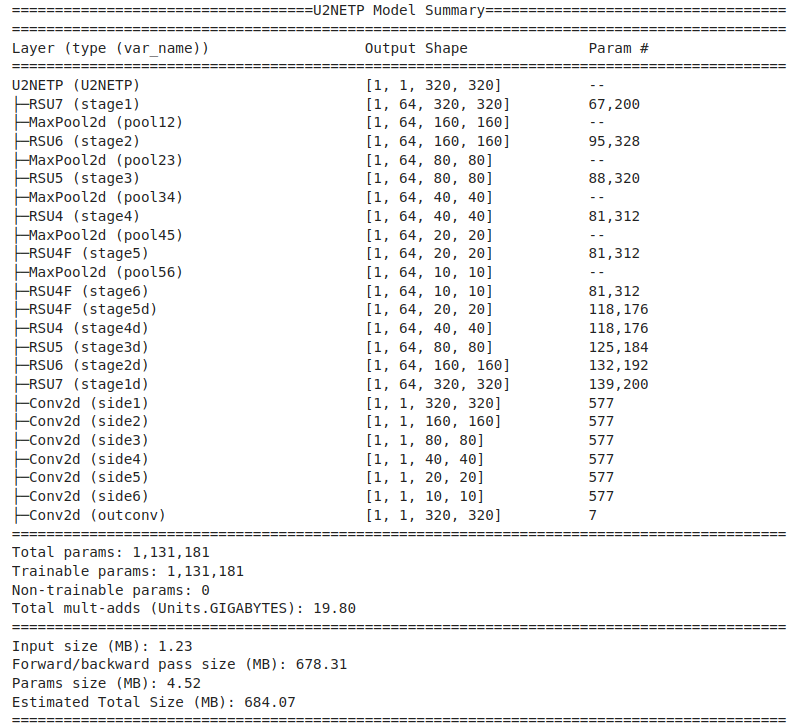
The U2NETP model is around 38 times smaller than the original U2-Net model, containing only around 1.13M parameters, as the model summary vindicates.
Next, we load the model weights using the load_model helper function.
def load_model(model, model_path, device):

    model.load_state_dict(torch.load(model_path, map_location=device))
    model = model.to(device)

    return model
The model weights are now loaded through the following lines of code.
u2net = load_model(model=u2net, model_path="u2net.pth", device="cuda:0")

u2netp = load_model(model=u2netp, model_path="u2netp.pth", device="cuda:0")
Data Preprocessing
Next, we shall prepare the batch image samples. The authors recommend resizing the image resolution to 320x320 during inference.
We will also scale the image data in the range [0, 1] and normalize it using the ImageNet mean and standard deviation.
mean = torch.tensor([0.485, 0.456, 0.406])
std = torch.tensor([0.229, 0.224, 0.225])

resize_shape = (320,320)

transforms = T.Compose([T.ToTensor(),
                        T.Normalize(mean=mean, std=std)])
Using the above transforms, we will prepare the batch data and provide the path to the image directory.
def prepare_image_batch(image_dir, resize, transforms, device):

    image_batch = []

    for image_file in os.listdir(image_dir):
        image = Image.open(os.path.join(image_dir, image_file)).convert("RGB")
        image_resize = image.resize(resize, resample = Image.BILINEAR)

        image_trans = transforms(image_resize)
        image_batch.append(image_trans)


    image_batch = torch.stack(image_batch).to(device)

    return image_batch

image_batch = prepare_image_batch(image_dir="test_images",
                                 resize=resize_shape,
                                 transforms=transforms,
                                 device="cuda:0")
We will provide a helper function to denormalize images in the range [0, 255]. This would be required for visualization purposes. The denorm_image utility denormalizes an image using the same ImageNet mean and standard deviation.
def denorm_image(image):
    image_denorm = torch.addcmul(mean[:,None,None], image, std[:,None, None])
    image = torch.clamp(image_denorm*255., min=0., max=255.)
    image = torch.permute(image, dims=(1,2,0)).numpy().astype("uint8")

    return image
Prepare Model Predictions
Once we have pre-processed our image batch, we can forward pass it through the model. The prepare_predictions utility does precisely this.
def prepare_predictions(model, image_batch):

    model.eval()

    all_results = []

    for image in image_batch:
        with torch.no_grad():
            results = model(image.unsqueeze(dim=0))

        all_results.append(torch.squeeze(results[0].cpu(), dim=(0,1)).numpy())

    return all_results
Let’s remember that the forward method for the U2NET model produces a combined (fused) probability map alongside separate side outputs. However, we’ll only be utilizing the fused prediction map.
We obtain the predictions for both the U2-Net and U2-NetP models.
predictions_u2net = prepare_predictions(u2net, image_batch)
predictions_u2netp = prepare_predictions(u2netp, image_batch)
Once we have the predictions, we can normalize them using the simple min-max normalization.
def normPRED(predicted_map):
    ma = np.max(predicted_map)
    mi = np.min(predicted_map)

    map_normalize = (predicted_map - mi) / (ma-mi)

    return map_normalize
We shall now visualize the model predictions for both U2Net and U2-NetP.
Let’s take a look at a simple example.
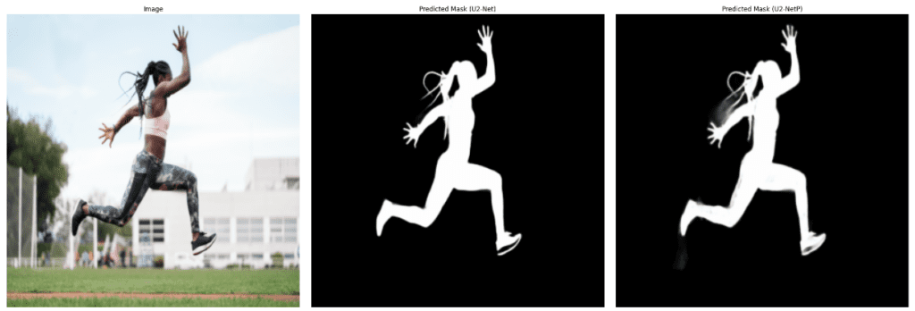
Both U2-Net (2nd column) and U2-NetP (3rd column) give decent predictions. However, U2-Net produces slightly better predictions around the sprinter’s hair portion.
The next series of predictions shows that U2-Net produces a higher-confidence probability map than its U-NetP counterpart.
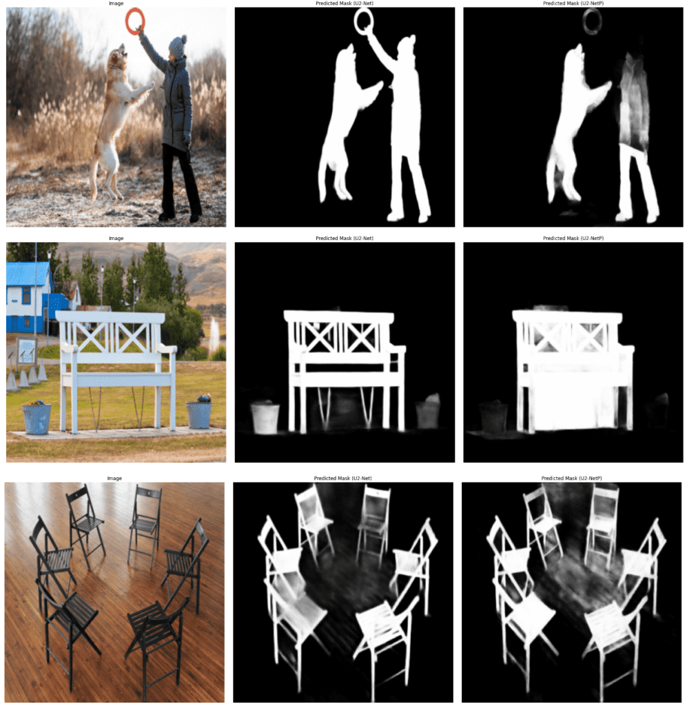
However, there are instances where U2-NetP surprisingly gives better prediction maps compared to U2-Net.
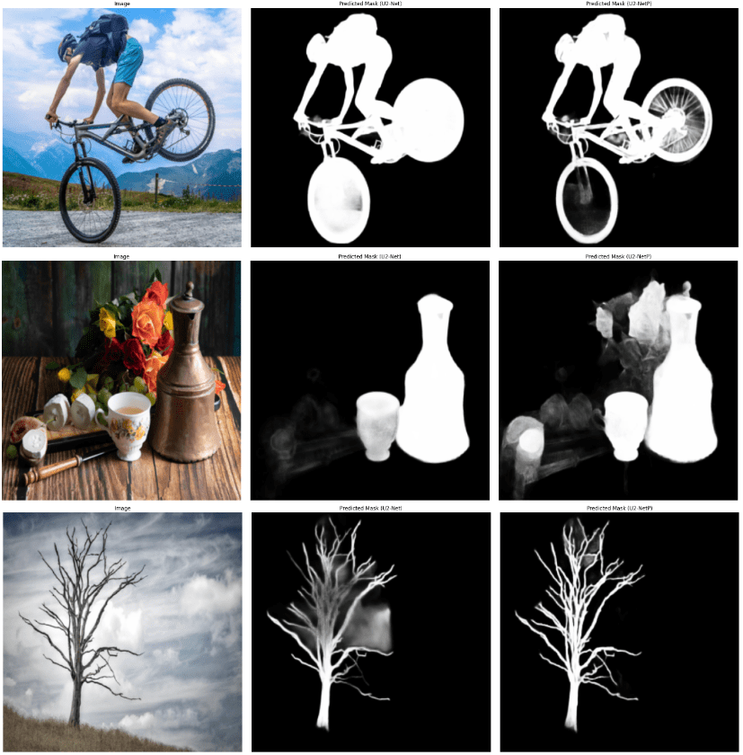
Let us now take a closer look at a few challenging examples.
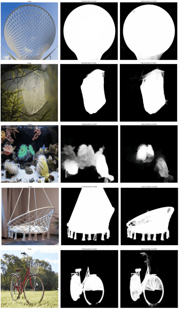
Although both models were able to segment out the foreground instances, there is tremendous scope for improvements in getting more fine-grained segmentation results.
The following section will discuss the IS-Net architecture composed of RSU blocks in the encoder-decoder stages. It is similar to the U2-Net structure but can produce significantly better results.
IS-Net Architecture: Advancing U2-Net for Image Segmentation
The authors of the U2-Net paper proposed a more robust approach to performing foreground segmentation using an efficient intermediate supervision (IS) learning strategy in their paper, “Highly Accurate Dichotomous Image Segmentation,” released in 2022.
There were three major highlights of the paper:
- Curation of the first large-scale dataset: DIS5K, containing 5470 high-resolution image data coupled with highly accurate binary segmentation masks.
- Implement an intermediate self-supervision strategy (IS) to learn a ground-truth mask-level encoder and incorporate it with the segmentation component (based on U2-Net) to learn mask-level and image-level features via feature synchronization. The entire architecture is referred to as IS-Net.
- Design of a novel metric called Human Correction Efforts (HCE) to approximate the number of mouse-clicking operations required to correct the false positives and false negatives.
We shall focus only on the IS-Net architecture since we intend to compare the inference results with the previous models.
The IS-Net architecture comprises two components:
- A ground truth encoder to learn high-dimensional mask-level encodings.
- An image segmentation component (similar to U2-Net) to learn high-resolution multi-stage and multi-level image features.
Note: Unlike U2-Net, the segmentation component doesn’t use a concatenated (fused) module of the side output maps.
The block diagram below shows the proposed IS-Net training pipeline.
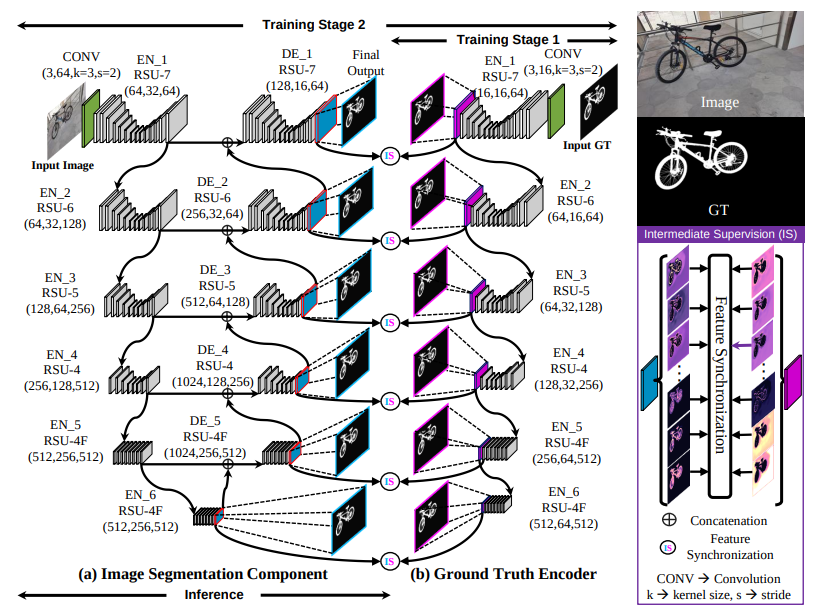
The training is performed with a 1024×1024 input image resolution. The authors employ a two-phase training pipeline which involves the following phases:
- The first phase involves training a self-supervised ground truth encoder model to learn high-dimensional mask-level features.
The encoder consists of 6-stage RSU encoder blocks (discussed earlier). Specifically, encoders from stages 1-4 employ the RSU-7, RSU-6, RSU-5, and RSU4 modules, respectively, while those from stages 5-6 use the RSU-4F modules.
Note: To reduce the computation cost, a downsampled version (512×512) of the high-resolution ground truth mask (1024×1024) is passed to the encoder stages through strided convolution (with a stride of 2).
The training involves using a simple binary cross-entropy loss involving the side output maps (a result of 3×3 convolutions on top of the encoder outputs across each stage) alongside the ground truth masks. - The image segmentation component consists of five decoder stages (DE_1-DE_5 employing the RSU7-RSU4F modules) and six encoder stages (EN_1 – EN_6 comprising RSU-7 to RSU-4F in that order).
This segmentation model produces the side output probability maps and the intermediate features (the logits without the sigmoid activations) from the decoder stages (DE_1 – DE_5) and the last encoder stage (EN_6).
The authors use an MSE (mean-squared error) loss between the learned encodings and the predicted output features from the decoder stages (devoid of the side outputs) to perform feature synchronization (FS) through intermediate supervision. The FS loss (Lfs) is formulated using:

Where,
- fdI is the image features (logits without activations) extracted from the decoder stage d (devoid of the side outputs) from the segmentation component.
- fdG is the mask-level encoding learned in the first training phase from encoder stage d.
- The weighting factor
 is kept as 1 for each stage.
 - D=6; representing the stages of the segmentation model (DE_1 – DE_5 and EN_6)
Additionally, the segmentation training process is identical to U2-net, which computes the standard BCE loss (Lsg) of the side outputs and the ground truth masks discussed in the [Loss and Optimizer for U2-Net Training section].
The training process for the segmentation component is perceived as the following optimizing problem:
![]()
We should remember that only the segmentation component of the IS-Net pipeline is used for inference, as we had done with the previous U2-Net models.
Inference Results from IS-Net
We will now perform inference on some image samples using the IS-Net pipeline, which contains a mix of easy and challenging instances. Finally, we will compare the results with U2-Net.
We will import the model architecture in the isnet.py script.
from isnet import ISNetDIS

isnet = ISNetDIS(in_ch=3,out_ch=1)
The IS-Net is a 44M parameter model similar to that of U2-Net. We can observe the model summary shown below.
Next, we load the model weights.
isnet = load_model(model=isnet, model_path="isnet-general-use.pth", device="cuda:0")
We will now use the following pre-processing transforms to the image data. We will perform the inference using the 1024x1024 image resolution suggested by the authors.
mean = torch.tensor([0.5, 0.5, 0.5])
std = torch.tensor([1.0, 1.0, 1.0])

resize_shape = (1024,1024)

transforms = T.Compose([T.ToTensor(),
                        T.Normalize(mean=mean, std=std)])
Since the IS-Net pipeline doesn’t use a fused side output map, we will use the side output from the first decoder stage (DE_1) for inference. The prepare_predictions utility remains largely the same, with the only difference being that we use the first side output (from the first decoder stage).
def prepare_predictions(model, image_batch):

    model.eval()

    all_results = []

    for image in image_batch:
        with torch.no_grad():
            results = model(image.unsqueeze(dim=0))

        all_results.append(torch.squeeze(results[0][0].cpu(), dim=(0,1)).numpy())

    return all_results
Let us visualize a couple of inference samples and compare them with those from U2-Net.
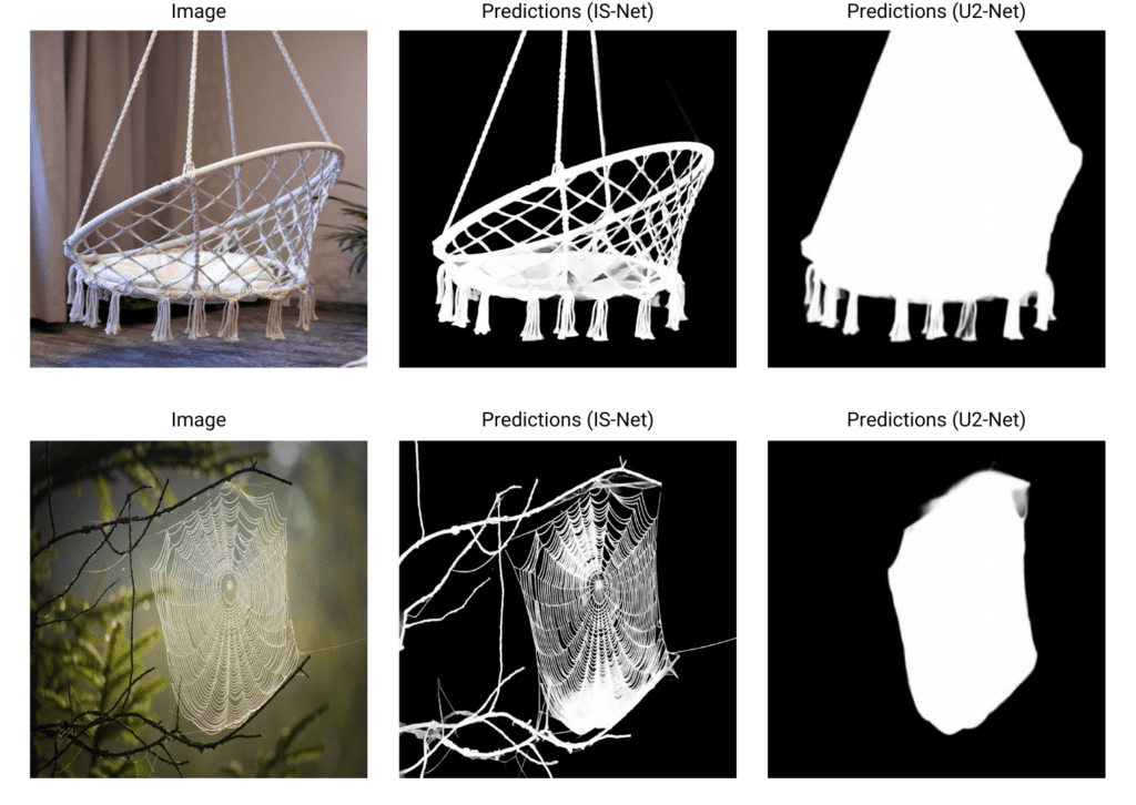
We can observe that IS-Net gives stunning results compared to its U2-Net counterpart.
Now, we look into a few more challenging instances.
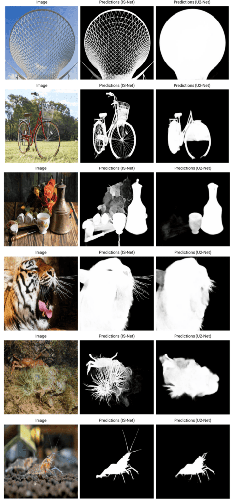
Did you find the results exciting? Jump to the RSU-block explanation section to know more about the U2-Net.
We might be tempted to believe that IS-Net always produces better prediction masks than U2-Net. That might be most of the time, but we show a few exceptions where U2-Net could give better prediction masks.
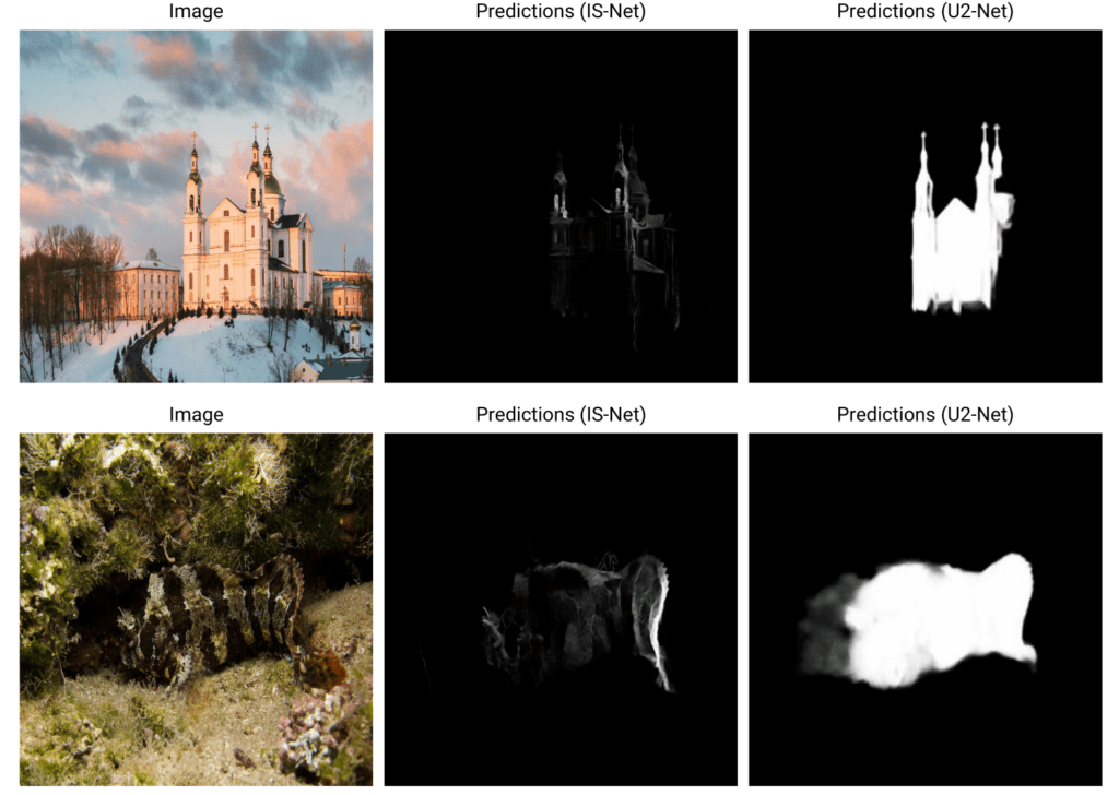
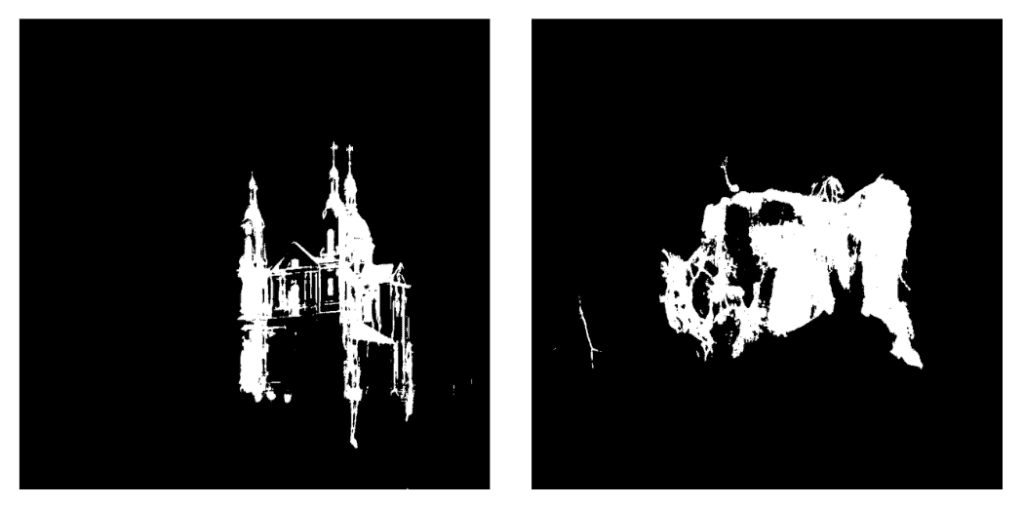
However, we can improve the IS-Net prediction masks by using OpenCV’s thresholding utility. We kept the thresholded values to 10.
Key Takeaways
- ReSidual-U block: We have learned how the ReSidual-U structure (RSU) pivots in learning multi-scale global context in addition to learning from local representations. It forms the crux of the pipeline for both U2-Net and IS-Net.
- U2-Net: The U2-Net is a nested two-level structure of RSU encoder-decoder layers that helps attain multi-level and multi-scale deep feature representations without requiring a pre-trained classification backbone at minimal computation and memory costs.
- Intermediate Supervision Strategy: Training a self-supervised ground-truth encoder from the target segmentation masks helps capture high-dimensional mask-level features.
- IS-Net pipeline: The IS-Net pipeline aims to attain feature synchronization using the trained GT encoder and the multi-stage feature maps, along with learning intra-stage and multi-level image features through the segmentation component (similar to U2-Net).
Conclusion
Background subtraction is one of the most crucial tasks in computer vision, and hence, understanding the high-dimensional multi-scale and multi-level image features is imperative. In this post, we have explored how U2-Net helps achieve this through its RSU blocks. We also observed that incorporating an intermediate supervision strategy results in significant improvements while generating the prediction masks, as evidenced by the IS-Net pipeline.
References
- U2-Net: Going Deeper with Nested U-Structure for Salient Object Detection
- Highly Accurate Dichotomous Image Segmentation (DIS)
- U2-Net Repository
- DIS repository
- DIS5K v1.0 Dataset




100K+ Learners
Join Free OpenCV Bootcamp3 Hours of Learning