YOLOv9 Instance Segmentation on Medical Dataset

Deep learning has revolutionized medical image analysis. By identifying complex patterns within medical images, it helps us to interpret crucial insights about our biological systems. So, if you ever have a desire to leverage deep learning for medical diagnostics, this article can be a good starting point for finetuning YOLOv9 Instance Segmentation on medical dataset.

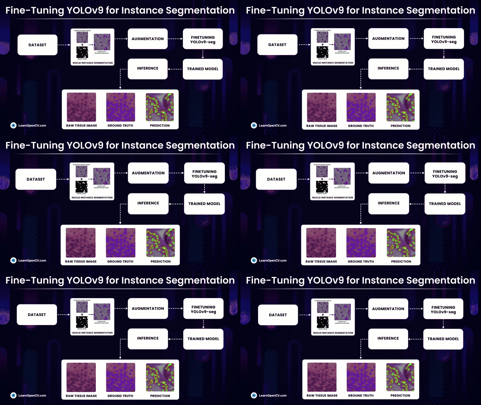
Rather than simply classifying regions as belonging to a particular cell type, Instance Segmentation models precisely localize and delineate the exact boundaries of individual cell instances. At first we will discuss, fine-tuning the latest YOLOv9 segmentation models on a custom medical dataset with Ultralytics and subsequently compare it against much refined YOLOv8-seg models.

For a quick glance at the experimental results, click here .

What is Instance Segmentation? 

Instance Segmentation involves classifying each pixel or voxel of a given image or volume to a particular class and assigning a unique identity to the pixels of individual objects. Semantic Segmentation, on the other hand, also classifies each pixel of an image to a particular class, but it does not differentiate between individual objects of the same class. All pixels belonging to a single class are assigned the same label, without distinguishing between different objects.

This makes Instance Segmentation suitable for applications where the outline of objects, their spatial distribution matter, and individual identities. So meticulously, Instance segmentation is a combination of object detection(class-wise localization)  and segmentation (pixel-wise classification).

YOLO Master Post –  Every Model Explained

Unlock the full story behind all the YOLO models’ evolutionary journey: Dive into our extensive pillar post, where we unravel the evolution from YOLOv1 to YOLO-NAS. This essential guide is packed with insights, comparisons, and a deeper understanding that you won’t find anywhere else.
Don’t miss out on this comprehensive resource, Mastering All Yolo Models for a richer, more informed perspective on the YOLO series.

Mastering All YOLO Models from YOLOv1 to YOLOv10: Papers Explained (2024)

Why YOLOv9 Instance Segmentation?

For lightweight models like YOLO and SSD, there is a risk of information degradation during the forward pass. Because, Information loss primarily occurs due to downsampling operations used within their architectures. 

These models rapidly reduce spatial dimensions through pooling and strided convolutions to compress the input image into a compact feature representation. While this helps to increase the receptive field and reduce the computational cost, it results in the loss of fine-grained details that are vital for detecting small and densely packed objects.

To address this, YOLOv9 leverages the Generalised Efficient Layer Aggregation Network ( GELAN) to achieve superior parameter utilization and computational efficiency. YOLOv9 primarily focuses on addressing the information loss in deep neural networks with Programmable Gradient Information (PGI) and Reversible Functions.

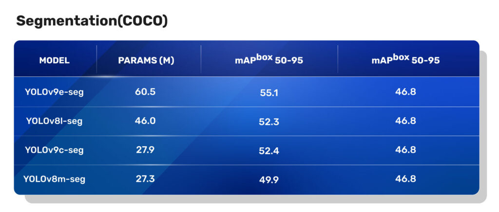
From this table, it is evident that the YOLOv9 instance segmentation models have a significant improvement in mAP on COCO Segmentation tasks compared to the YOLOv8 segmentation models.

For an in-depth understanding of YOLOv9 architecture, give a quick read on Fine Tuning YOLOv9 for object detection.

Understanding the Dataset for YOLOv9 Instance Segmentation

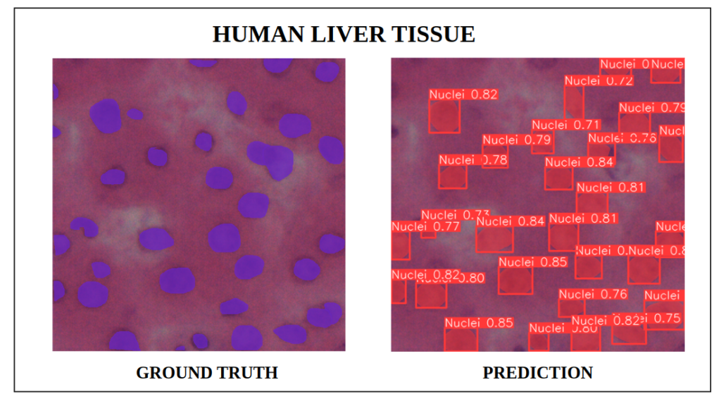
Nuclei Instance Segmentation Dataset: Visualization

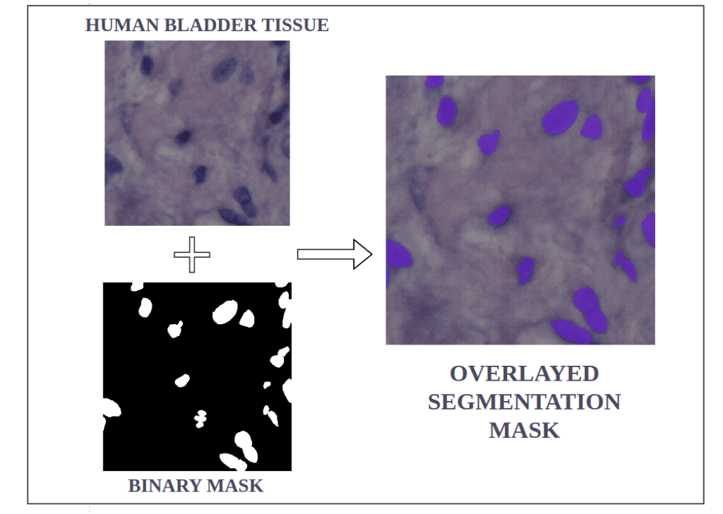
Medical expertise plays an indispensable role in enhancing model generalizability across different imaging modalities. This is achieved through meticulously curating high-quality annotated datasets and expert guidance throughout the model training and evaluation phases.

So, we will make use of one such high-quality medical NuInsSeg Kaggle dataset that contains more than 30k manually segmented nuclei from 31 human and mouse organs and 665 image patches extracted from H&E-stained whole slide microscopic images. 

The dataset contains tissues of various human and mouse organs. Key Human and Mouse organs include the cerebellum, kidney, liver, pancreas, etc.

The dataset contains a single Nuclei class and 665 images in total. Let’s split it with an 80:20 train val split ratio.

Then, the final split has 532 training and 133 validation images, respectively.
All the images are of dimension 512 x 512.

To access the code featured in this article and try fine-tuning it yourself, simply fill details in the “Download Source Code” banner.

Click here to download the source code to this post

Code Walkthrough

Recently, YOLOv9 Instance Segmentation models have been integrated into the Ultralytics package. We will make use of it to set up our training pipeline.

!pip install -q ultralytics pycocotools scikit-learn matplotlib 

Let’s install the necessary packages required to convert our dataset into YOLO format. Here, pycocotools for evaluation metrics, and scikit-learn splits the dataset into train and validation.

import os
import copy
import random
import json
import yaml
import glob
import cv2
import numpy as np
import time
import matplotlib.pyplot as plt
import matplotlib.patches as patches
import requests
from   zipfile import ZipFile
import argparse
from PIL import Image
import PIL.Image
import shutil
from IPython.display import Image
from sklearn.model_selection import train_test_split

import torch
import torch.utils.data
from torch import nn
import torchvision
from torchvision import transforms as T

from ultralytics import YOLO

Let’s set seed for reproducibility.

def set_seeds():
    # fix random seeds
    SEED_VALUE = 42

    random.seed(SEED_VALUE)
    np.random.seed(SEED_VALUE)
    torch.manual_seed(SEED_VALUE)
    
    if torch.cuda.is_available():
        torch.cuda.manual_seed(SEED_VALUE)
        torch.cuda.manual_seed_all(SEED_VALUE)
        torch.backends.cudnn.deterministic = True
        torch.backends.cudnn.benchmark = True
set_seeds()

Download the Dataset

This function block is used to download and unzip the dataset in the specified directory.

def download_and_unzip(url, save_path, extract_dir):
    print("Downloading assets...")
    file = requests.get(url)
    open(save_path, "wb").write(file.content)
    print("Download completed.")

    try:
        if save_path.endswith(".zip"):
            with ZipFile(save_path, 'r') as zip_ref:
                zip_ref.extractall(extract_dir)
            print("Extraction Done")
    except Exception as e:
        print(f"An error occurred: {e}")

DATASET_URL = r"https://www.dropbox.com/scl/fi/u83yuoea9hu7xhhhsgp4d/Nuclei_Instance_Seg.zip?rlkey=7tw3vs4xh7rych4yq1xizd8mh&dl=1"
DATASET_DIR = "Nuclei-Instance-Dataset"
DATASET_ZIP_PATH = os.path.join(os.getcwd(), f"{DATASET_DIR}.zip")

# Download and extract if dataset does not exist.
if not os.path.exists(DATASET_DIR):
    os.makedirs(DATASET_DIR, exist_ok=True)  # Ensure the directory exists
    download_and_unzip(DATASET_URL, DATASET_ZIP_PATH, DATASET_DIR)
    os.remove(DATSET_ZIP_PATH)  # Remove the zip file after extraction

Remove Unwanted Directories

The dataset comes with many subdirectories. However, for our YOLOv9 instance segmentation fine-tuning, we just need the raw images and labeled masks, and convert them to the appropriate format.

def prune_subdirectories(base_dir,keep_dirs):
    #Iterate through each subdirs in base dir
    for root_dir in os.listdir(base_dir):
        root_path = os.path.join(base_dir,root_dir)
        if os.path.isdir(root_path):
          #  print(f"Processing: {root_path}")
           #List all subdirs inside the current root dir
           for sub_dir in os.listdir(root_path):
               sub_path = os.path.join(root_path, sub_dir)
               #If the subdirectory isn't in the keep list, delete it
               if os.path.isdir(sub_path) and sub_dir not in keep_dirs:
                  # print(f"Deleting: {sub_path}")
                  shutil.rmtree(sub_path)
               elif os.path.isdir(sub_path):
                  # print(f"Keeping: {sub_path}")
                  pass

base_directory = "./Nuclei-Instance-Dataset"
directories_to_keep = ['tissue images', 'mask binary witthout border', 'label masks modify']

prune_subdirectories(base_directory,directories_to_keep)

For our task, just keep the directories with subdirectories named ‘tissue images’ , ‘mask binary without border’, and ‘label masks modify’.
After pruning, our dataset tree will look like this:

Nuclei-Instance-Dataset
├── human bladder
│   ├── label masks modify
│   └── tissue images
├── human brain
│   ├── label masks modify
│   └── tissue images
├── human cardia
│   ├── label masks modify
│   └── tissue images
├── human cerebellum
│   ├── label masks modify
│   └── tissue images
├── …
│   ├── label masks modify
│   └── tissue images
└── mouse thymus
    ├── label masks modify
    └── tissue images

Further, let’s try to convert our annotations from binary masks to YOLO format. As an intermediate step, let’s convert them to COCO JSON format, which is easy to interpret.

YOLOv9 Instance Segmentation Utility Functions

The get_image_mask_pairs() returns all image and mask paths from the dataset, appended to a list.

def get_image_mask_pairs(data_dir):
    image_paths = []
    mask_paths = []

    for root,_,files in os.walk(data_dir):
        if 'tissue images' in root:
            for file in files:
                if file.endswith('.png'):
                    image_paths.append(os.path.join(root,file))
                    mask_paths.append(os.path.join(root.replace('tissue images','label masks modify'), file.replace('.png','.tif')))
    return image_paths, mask_paths

Binary masks are a common way to represent object annotations in segmentation tasks. They efficiently encode the shape of objects at the pixel level. However, it is often beneficial to convert these masks into polygons for tasks like visualization or calculating object properties. The mask_to_polygons() shows one such approach to extract polygons from a binary mask.

def mask_to_polygons(mask,epsilon=1.0):
    contours,_ = cv2.findContours(mask,cv2.RETR_TREE,cv2.CHAIN_APPROX_SIMPLE)
    polygons = []
    for contour in contours:
        if len(contour) > 2:
           poly = contour.reshape(-1).tolist()
           if len(poly) > 4: #Ensures valid polygon
              polygons.append(poly)
    return polygons

We need to convert our tissue’s binary mask to actionable polygon points. For this, let’s use cv2.findContours to extract approximate polygons of the binary mask. This ensures we get a valid closed polygon with more than 4 sides and outlines around mask borders. By using cv2.RETR_TREE as contour retrieval mode, we can reconstruct a hierarchical relationship between all the detected contours.

This article on contour detection, will help you have a comprehensive view of the concept.

YOLO Annotation Format

Before continuing with the code, let’s take a moment to understand the YOLO annotation format for the instance segmentation task. In YOLO Instance segmentation format, annotations are stored in a separate .txt file corresponding to each image, with both image and annotation files sharing the same base filename.

For example, the image human_kidney01.png should have a matching annotation file named human_kidney01.txt.

Each row in a .txt file corresponds to a single object instance found in that associated image file.

Each row contains the following information about an instance:
Object Class Index: An integer referring to the object’s class index (e.g., 0 for Nuclei).

Object Bounding Coordinates: These are the normalized bounding coordinates around the object’s segmented area, ensuring that annotations are scalable across images of different dimensions.
Therefore, each row in a .txt file would look like
<class-index> <x1> <y1> <x2> <y2> … <xn> <yn>

Dataset Preparation

The process_data utility, will initialize annotation and images as empty lists to which all the metadata will be appended. Additionally, image ID and ann ID will have zero as initial values.

Next, simultaneously iterate through the image_paths and mask_path list, obtained from the get_image_mask_pairs utility function. For each image,  assign a unique image_id by incrementing with 1 after each iteration. Then, read the image and mask using OpenCV. The cv2.IMREAD_UNCHANGED helps to read masks, including an alpha channel if present.

At first, assign the key information about each image, such as image_id, width, height, filename, etc., as a dictionary and append it to the images list.

def process_data(image_paths, mask_paths, output_images_dir, output_labels_dir):
    annotations = []
    images = []
    image_id = 0
    ann_id = 0

    for img_path, mask_path in zip(image_paths, mask_paths):
        image_id += 1
        img = cv2.imread(img_path)
        mask = cv2.imread(mask_path, cv2.IMREAD_UNCHANGED)
        shutil.copy(img_path, os.path.join(output_images_dir, os.path.basename(img_path)))

        # Add image to the list
        images.append({
            "id": image_id,
            "file_name": os.path.basename(img_path),
            "height": img.shape[0],
            "width": img.shape[1]
        })

        unique_values = np.unique(mask)

Mask to Polygons

This snippet discusses how to use np.unique(mask) function to find distinct pixel values within a mask image and demarcate distinct objects within a mask. Subsequently, it loops over each unique value identified. For each value of an object (ignoring background), a binary mask is constructed where pixels corresponding to the current unique value are set to 255 (white) to highlight the object instance. 

While all other pixels are set to 0 (black) effectively isolating the object from the background. The binary mask is then passed as input to the mask_to_polygons() function, which processes the mask and returns a series of polygons.

for value in unique_values:
            if value == 0:  # Ignore background
                continue

            object_mask = (mask == value).astype(np.uint8) * 255
            polygons = mask_to_polygons(object_mask)

            for poly in polygons:
                ann_id += 1
                annotations.append({
                  
                    "image_id": image_id,
                    "category_id": 1,  # Only one category: Nuclei
                    "segmentation": [poly],  
                })

Each polygon outlines the perimeter of an object within the mask, providing the necessary data for accurate instance segmentation. Now, iteratively, each polygon is assigned a unique ann_id. The necessary annotation information for the segmentation task is appended as a dictionary to the annotations list.

COCO to YOLO Format Conversion

 coco_input = {
        "images": images,
        "annotations": annotations,
        "categories": [{"id": 1, "name": "Nuclei"}]
    }

And now our annotations are already in COCO json format. Following this, convert the COCO annotations to YOLOv9 Instance Segmentation format methodically.

 # Convert COCO-like dictionary to YOLO format
    for img_info in coco_input["images"]:
        img_id = img_info["id"]
        img_ann = [ann for ann in coco_input["annotations"] if ann["image_id"] == img_id]
        img_w, img_h = img_info["width"], img_info["height"]

        if img_ann:
            with open(os.path.join(output_labels_dir, os.path.splitext(img_info["file_name"])[0] + '.txt'), 'w') as file_object:
                for ann in img_ann:
                    current_category = ann['category_id'] - 1
                    polygon = ann['segmentation'][0]
                    normalized_polygon = [format(coord / img_w if i % 2 == 0 else coord / img_h, '.6f') for i, coord in enumerate(polygon)]
                    file_object.write(f"{current_category} " + " ".join(normalized_polygon) + "\n")

For this, iterate over the coco_input dictionary for each image, and retrieve its unique identifier (img_id) and associated annotations (img_ann) from the annotations list.

Now, for each image, a corresponding .txt annotation file is created, category_id is extracted and polygon of the current object instance in a recurring loop. The polygon is then normalized with relative to the current image dimensions. Thus, a set of .txt files for all images is created in the output labels dir, which will be utilized during fine-tuning.

 Preparing data.yaml

We will dump the required data set in a separate data.yaml file to fit our training pipeline for any YOLO models. This file contains the paths for train, validation, and test image directories along with the names of classes and the number of classes in the dataset.

def create_yaml(output_yaml_path, train_images_dir, val_images_dir, nc=1):
    # Assuming all categories are the same and there is only one class, 'Nuclei'
    names = ['Nuclei']

    # Create a dictionary with the required content
    yaml_data = {
        'names': names,
        'nc': nc,  # Number of classes
        'train': train_images_dir,
        'val': val_images_dir,
        'test': ' '
    }
    # Write the dictionary to a YAML file
    with open(output_yaml_path, 'w') as file:
        yaml.dump(yaml_data, file, default_flow_style=False)

The dataset dir should have the following tree structure:

yolov9_1024_dataset
├── train
│   ├── images
│   │   ├── human_kidney01.png  
│   │   └── ...                 
│   └── labels
│       ├── human_kidney01.txt   
│       └── ...                 
└── val
    ├── images
    │   ├── human_kidney01.png  
    │   └── ...                 
    └── labels
        ├── human_kidney01.txt  
        └── ...  

Now, the yolo_dataset_preparation() function defines all the paths and then calls the required set of utility functions. To simply put, this function is responsible for extracting the polygons from the raw binary masks and converting them into YOLO format. Finally, it creates a data.yaml file for the YOLOv9 Instance Segmentation finetuning.

def yolo_dataset_preparation():
    data_dir = 'Nuclei-Instance-Dataset'
    output_dir = 'yolov9e_1024_dataset'

    # Define the paths for the images and labels for training and validation
    train_images_dir = os.path.join(output_dir, 'train', 'images')
    val_images_dir = os.path.join(output_dir, 'val', 'images')
    train_labels_dir = os.path.join(output_dir, 'train', 'labels')
    val_labels_dir = os.path.join(output_dir, 'val', 'labels')

    # Create the output directories if they do not exist
    os.makedirs(train_images_dir, exist_ok=True)
    os.makedirs(val_images_dir, exist_ok=True)
    os.makedirs(train_labels_dir, exist_ok=True)
    os.makedirs(val_labels_dir, exist_ok=True)

    # Get image and mask paths
    image_paths, mask_paths = get_image_mask_pairs(data_dir)

    # Split data into train and val
    train_img_paths, val_img_paths, train_mask_paths, val_mask_paths = train_test_split(image_paths, mask_paths, test_size=0.2, random_state=42)

    # Process and save the data in YOLO format for training and validation
    process_data(train_img_paths, train_mask_paths, train_images_dir, train_labels_dir)
    process_data(val_img_paths, val_mask_paths, val_images_dir, val_labels_dir)

    # Assume create_yaml function is defined elsewhere and set appropriate paths for the YAML file
    output_yaml_path = os.path.join(output_dir, 'data.yaml')
    train_path = os.path.join('train', 'images')
    val_path = os.path.join('val', 'images')
    create_yaml(output_yaml_path, train_path, val_path)

yolo_dataset_preparation()

YOLOv9 Instance Segmentation Model Setup

The Ultralytics package, have two YOLOv9 instance segmentation models.

Further on, we will be finetuning both YOLOv9e-seg  and YOLOv9c-seg and compare them against the equivalent parameter sized YOLOv8l-seg and YOLOv8m-seg models, respectively, for varying image size.

#Instance
model = YOLO("yolov9e-seg.yaml") #build a model from YAML
model = YOLO("yolov9e-seg.pt") #Transfer the weights from a pretrained model 

In this experiment, we’ll use a pre-trained YOLOv9e-seg model weights on the COCO dataset with all layers unfreezed.

However, you can also experiment with,

• YOLOv9 Instance Segmentation: Fine Tuning with Partially Frozen Layers –
  • Freeze the model’s backbone layers, which are responsible for generable feature extraction, and only unfreeze the YOLOv9-seg head layers specialized for segmentation.
• YOLOv9 Instance Segmentation: Transfer Learning –
  • Completely freeze the pre-trained YOLOv9e-seg model and only train the final head layer specific to the dataset for the segmentation task.

The below code snippet reads the data.yaml and fetches the number of classes of the training dataset.

with open("yolov9e_1024_dataset/data.yaml",'r') as stream:
     num_classes = str(yaml.safe_load(stream)['nc'])

Model Training

#Define a project --> Destination directory for all results
project = "yolov9e_1024_dataset/results"
#Define subdirectory for this specific training
name = "70_epochs-"
ABS_PATH = os.getcwd()

Let us train our models for 70 epochs and save the training logs into a specified project directory.

#Train the model
results = model.train(
    data = os.path.join(ABS_PATH, "yolov9e_1024_dataset/data.yaml"),
    project = project,
    name = name,
    epochs = 70,
    patience = 0 , #setting patience=0 to disable early stopping,
    batch = 3,
    imgsz=1024
)

Now, let’s start training by setting the model to training mode using the model.train(). We will finetune our YOLOv9e-seg model with a batch size of 3 and an image size of 1024, so that it fits into the GPU memory.

NOTE: If you encounter a CUDA out-of-memory (OOM) error, try reducing batch and image size accordingly for effective GPU memory utilization.

To ensure the model trains adequately and achieves optimal performance in terms of accuracy or minimal loss, setting patience to 0 deactivates early stopping.

Hardware Specification:

The training has been carried out on a RTX 4090 GPU with 24 GB vRAM and  AMD Ryzen 7532 32 cores 128 threads CPU.

To train with a Colab T4 free tier (Intel Xeon(R) @2.00Ghz single core 2 Threads per core), you can set the batch size to 4 and reduce the image size to 640x640.

Let’s set up our training and monitor the Ultralytics training logs. By observing the Ultralytics logs, one can get nuanced insights into how the default augmentations, Automatic Mixed Precision(AMP), and optimizer configuration are auto-applied.

For an Instance Segmentation task, it’s important to observe the primary mAP (i.e. mAP50-95) metric for both bounding box and segmentation.

To learn more about mAP, refer to our blog post on mAP metrics.

Training Summary

We can also live monitor the logs using tensorboard and observe how the finetuning persists.

%load_ext tensorboard
%tensorboard --logdir yolov9e_1024_dataset/results/70_epochs-

Let’s look at the results.png saved at “yolov9e_1024_dataset/results/70_epochs-/results.png”. The Ultralytics training summary and results.png gives an overall idea of how the model fine-tuning has been.

For YOLOv9e-seg Instance Segmentation with an imgsz=1024 training for 70 epochs, we achieved a validation box mAP50-95 of about 0.506 and validation seg mAP50-95 of about 0.457.

YOLOv9 Instance Segmentation Inference

The best model weight is loaded and let’s perform inference on few tissue samples.

inference_model = YOLO('yolov9e_1024_dataset/results/70_epochs-/weights/best.pt')

%matplotlib inline
inference_img_path = "yolov9e_1024_dataset/val/images/human_spleen_13.png"
inference_result = inference_model.predict(inference_img_path,conf=0.7,save=True,imgsz=1024)

print(inference_result)

print("Boxes:   \n",inference_result[0].boxes)

print("Masks:  \n",inference_result[0].masks)

inference_result_array = inference_result[0].plot() #Ultralytics plot function.
plt.figure(figsize=(9,9))
plt.imshow(inference_result_array)
plt.show()

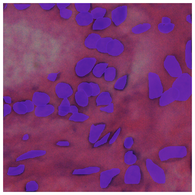
We can observe that for the above results, our fine-tuned YOLOv9e-seg model with a confidence score threshold of 0.7, was almost able to capture all instances with only 3 to 4 corner instances left undetected.
All the inference is done on (512,512) image dimension and conf=0.7, where the img size automatically resizes to the model’s training configuration. In Ultralytics default imgsz is 640x640.

So when we perform inference using YOLOv9e-seg model trained with an imgsz=1024, our input image automatically resizes to 1024. The input dimension during the forward pass will look like (1,3,1024,1024), where batch size = 1 and channel dimension = 3.
The inference_result is a dictionary with keys and values as follows:

• boxes: an object of dtype=float32, representing detected bounding box instances. The boxes have the following key attributes:
  • cls:  a tensor showing class names of all detected objects.
  • conf:  a tensor showing on what confidence the model, has detected those object instances.                  
  • Bounding Box formats(xywh, xywhn, xyxy, xyxyn): a tensor having normalized coordinate positions of instances in the inference image.
•  keypoints: None (for Instance Segmentation task).
•  masks: an object representing detected mask instances. The masks have the following key attributes:
  • xy:  an array of dtype=float32, having each mask’s polygon points location.
• names : class mapping of the dataset on which the model is trained.

YOLOv9 Instance Segmentation Custom Plotting Function

One can directly use the Utralytics plot() function for ease of use. However, extracting the masks, boxes, and class names and performing custom plotting is intuitively more beneficial. So, let’s have a look at the custom plotting by making use of the inference_result dictionary.

We will filter out detections by thresholded_indices with a confidence of more than 0.5. From the outputs, for all predicted instances extract the mask and box attributes.

def get_outputs(image, model, threshold=0.5):
    
    # print("Image shape",image.shape)
    outputs = model.predict(image, imgsz=1024, conf=threshold)
    print("Outputs",outputs)

    scores = outputs[0].boxes.conf.detach().cpu().numpy()
    thresholded_indices = [idx for idx, score in enumerate(scores) if score > threshold]
    print(f"Total detections: {len(scores)}, Passed threshold: {len(thresholded_indices)}")

    if len(thresholded_indices) > 0:
        masks = [outputs[0].masks.xy[idx] for idx in thresholded_indices]
        boxes = outputs[0].boxes.xyxy.detach().cpu().numpy()[thresholded_indices]
        boxes = [[(int(box[0]), int(box[1])), (int(box[2]), int(box[3]))] for box in boxes]
        labels = [outputs[0].names[int(outputs[0].boxes.cls[idx])] for idx in thresholded_indices]
    else:
        masks, boxes, labels = [], [], []

    return masks, boxes, labels

Segmentation Mapping

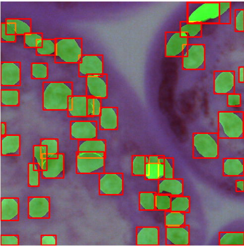
The draw_segmentation_map() function overlays, extracted predicted masks and bounding boxes on to the input image with cv2.fillPoly() and cv2.addWeighted().

def draw_segmentation_map(image, masks, boxes, labels):
    alpha = 1.0
    beta = 0.5  # Transparency for the segmentation map
    gamma = 0  # Scalar added to each sum
    image = np.array(image)  # Convert the original PIL image into a NumPy format
    image = cv2.cvtColor(image, cv2.COLOR_RGB2BGR)  # Convert from RGB to OpenCV BGR format

    for mask, box, label in zip(masks, boxes, labels):
        color = (0, 255, 0)  # Green color for visualization
        segmentation_map = np.zeros_like(image)

        if mask is not None and len(mask) > 0:
            poly = np.array(mask, dtype=np.int32)
            cv2.fillPoly(segmentation_map, [poly], color)

        cv2.addWeighted(image, alpha, segmentation_map, beta, gamma, image)
        cv2.rectangle(image, box[0], box[1], color=(255, 0, 0), thickness=2)  # Red color for bounding box

    return image

Save the output at a specified directory, using cv2.imwrite().

fig = plt.figure(figsize=(5, 5), layout="constrained")
image_path = "yolov9e_1024_dataset/val/images/human_placenta_24.png"
image = PIL.Image.open(image_path)
orig_image = image.copy()  # Keep a copy of the original image for OpenCV functions and applying masks

masks, boxes, labels = get_outputs(image, inference_model, threshold=0.5)
result = draw_segmentation_map(orig_image, masks, boxes, labels)

save_path = f"./inference/nuclei_instance_out{image_path.split(os.path.sep)[-1].split('.')[0]}.jpg"
cv2.imwrite(save_path, result)

plt.imshow(result)

plt.axis('off')
plt.show()

YOLOv9 Instance Segmentation Training Summary

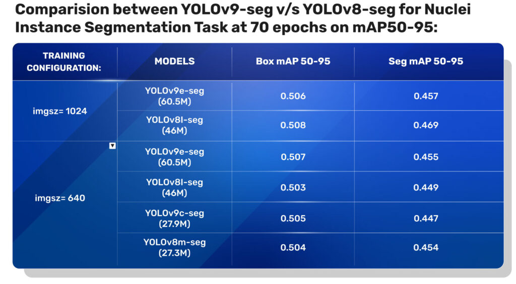
From Table 2, we observe that the validation box mAP and seg mAP for both YOLOv9 seg and YOLO V8 seg are nearly the same, with a slight difference in decimal precision.

Comparsion 1 : YOLOv9e-seg v/s YOLOv8l-seg with imgsz=1024

Let’s plot the validation box and seg mAP (50-95) of both models.

From the above chart, it is observed that for a training configuration of imgsz=1024 ,

• Compared to the YOLOv9e-seg models the YOLOv8l-seg model starts its baseline mAP, relatively higher and achieves higher mAP within fewer epochs.
• Also, the YOLOv8l-seg model’s box mAP and seg mAP are marginally higher than the YOLOv9e-seg.

Now, let’s do an in-depth comparison for a confidence score threshold of 0.7.

With respect to the ground truth, the green boxes are instances where the YOLOv9e-seg model failed to detect object instances.

Similarly, the yellow boxes are the object instances which the YOLOv8l-seg model didn’t not detect.

NOTE: Here, in the comparisons below, the green and yellow boxes are not bounding boxes of a predicted segments; rather, they are just decorations. These were manually drawn as references for us to understand the differences that the model failed to capture with respect to the Ground Truth.

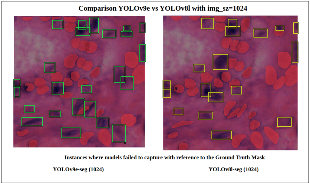
In this particular image of imgsz=1024 and conf=0.7, we can observe that YOLOv9e-seg missed 24 instances while the YOLOv8l-seg missed 18 instances.

i.e. YOLOv8l-seg performed better here.

Quantative Analysis with respect to Ground Truth

Now, let’s break down the quantitative differences in detection between both models in a specific region with blue boxes.

NOTE: Here, in the comparison below, the blue boxes are not bounding boxes of a predicted instances; rather, they are just decorations manually drawn to show the difference with respect to the Ground Truth.

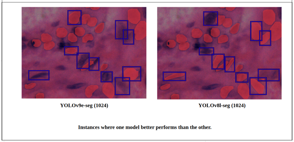
We again observe that the YOLOv8l-seg detects much more instances than the YOLOv9e-seg. When the image size is increased to 1024, YOLOv9e-seg perform relatively bad, but on contrary, increasing image size made the YOLOv8l-seg to perform better.

Comparison 2 : YOLOv9e-seg v/s YOLOv8l-seg with imgsz=640

Let’s plot the validation box and seg mAP(50-95) of both models.

From the above chart, it is observed that for a training configuration of imgsz=640 ,

• Compared to YOLOv9e-seg models, the YOLOv8l-seg model starts its baseline mAP relatively higher and achieves higher mAP within fewer epochs.
• Here, at the end of training, both models have nearly the same validation box mAP and seg mAP.

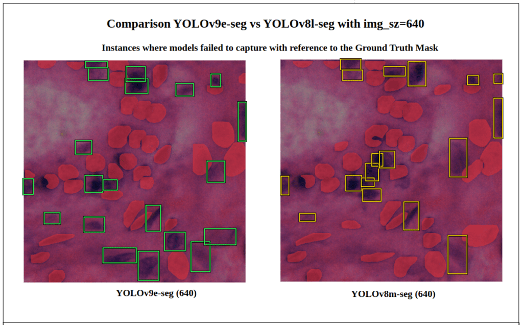
• We can observe in this particular image that YOLOv9e-seg (green) missed 20 instances while the YOLOv8l-seg (yellow) missed 18 instances with conf=0.7.
• i.e. YOLOv8l-seg performed better here and had fewer False Negatives.

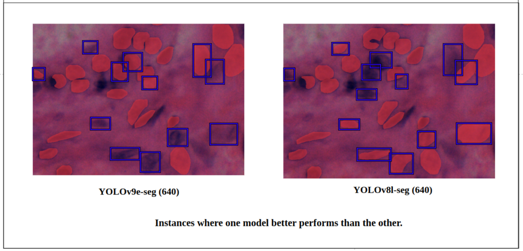
Let’s focus on a particular region of the tissue image. Both perform nearly the same, but YOLOv8l-seg is slightly better, with more True Positives.

Comparison 3 : YOLOv9c-seg v/s YOLOv8m-seg with imgsz=640

Let’s plot the validation box and seg mAP(50-95) of both models.

From the chart, it is observed that for a training configuration of imgsz=640,

• Compared to the YOLOv9c-seg model, the YOLOv8m-seg model starts its baseline mAP relatively higher and achieves higher mAP within fewer epochs.
• At the end of training, both models had nearly the same validation mAP.

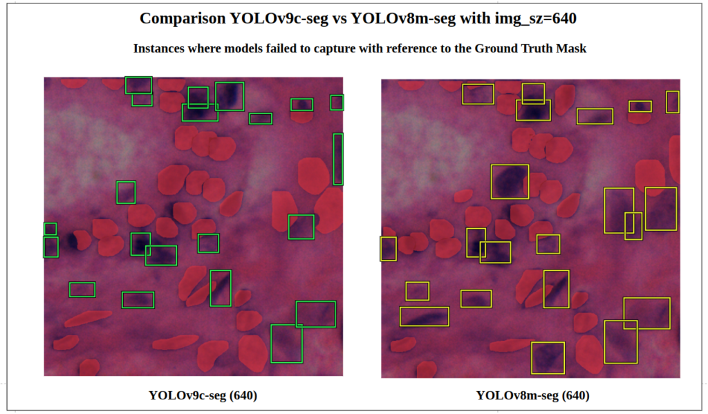
We can observe for this particular image that YOLOv9c-seg (green) missed 21 instances while the YOLOv8m-seg (yellow) missed 21 instances for conf=0.7.

Now, let’s break down the difference in existing detection between both models in a specific region.

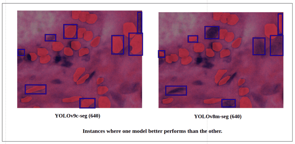
Here, for this particular region it is observe that , the YOLOv9c-seg detects much more True Positive instances than the YOLOv8m-seg.

YOLOv9 Instance Segmentation Prediction on Multiple Images

To better understand about all the models segmentation mask’s precision, let’s infer an extensive set of human tissue image predictions from the validation set. During inference to view predictions without bounding boxes, pass boxes=False argument. We will visualize all the predictions of both YOLOv9 and YOLOv8 models that we have experimented side by side with varying image size and confidence score threshold to 0.7, and compare predicted segmentation masks.

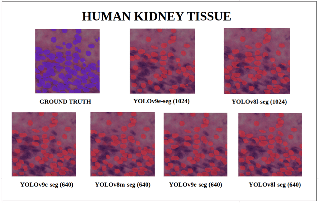
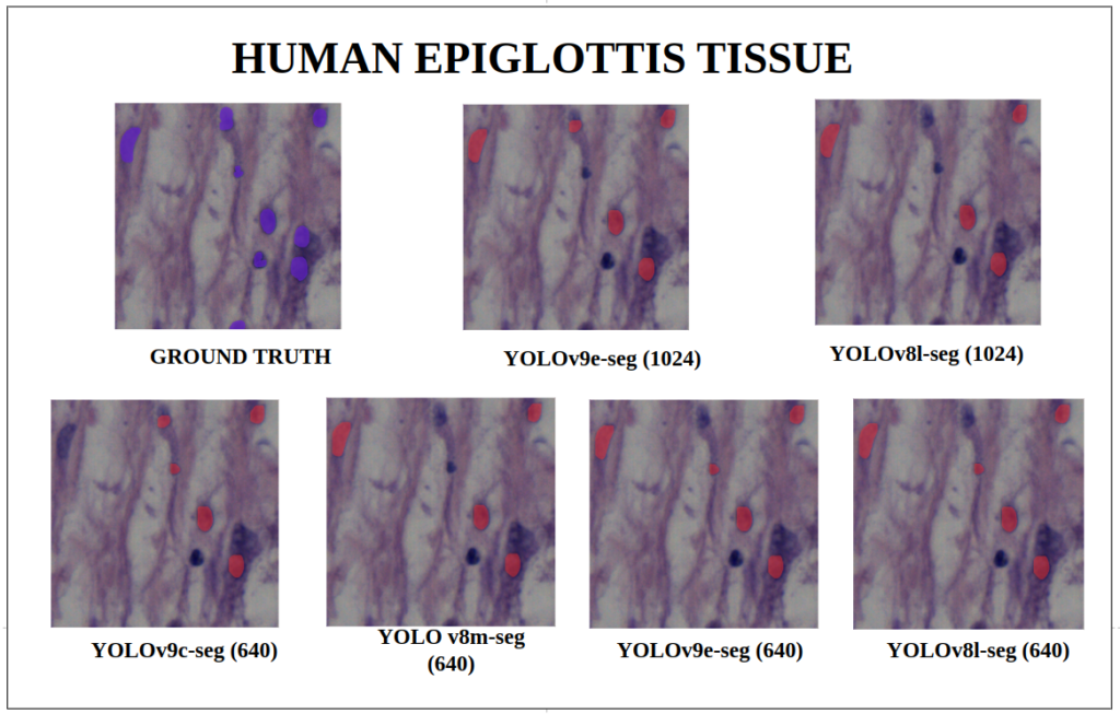
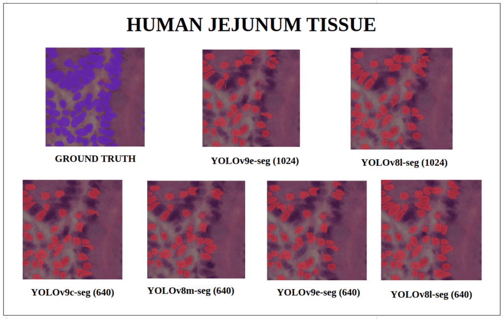
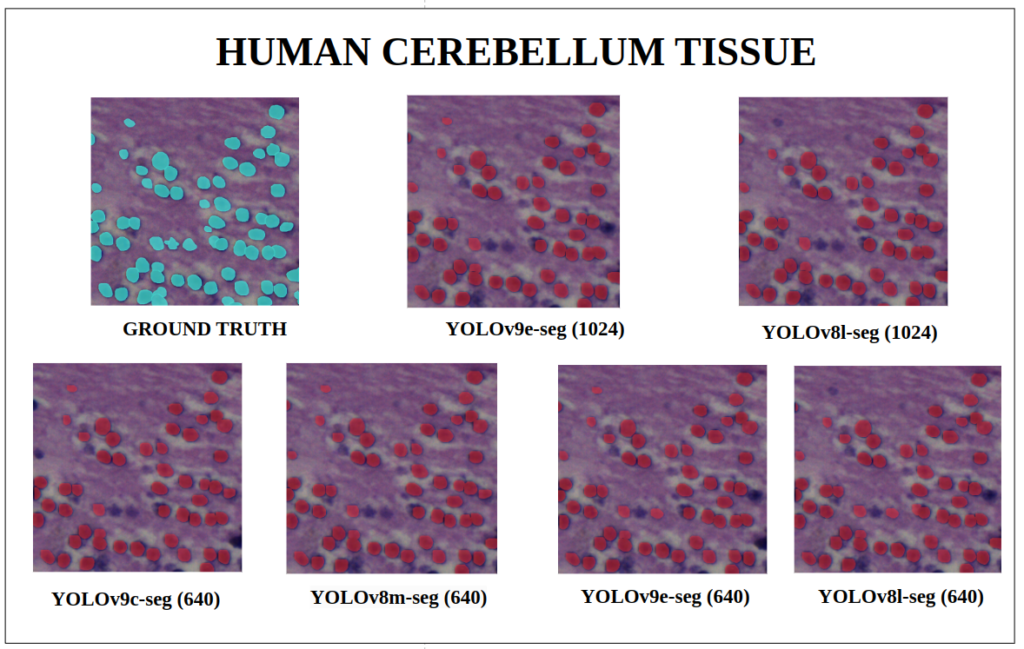
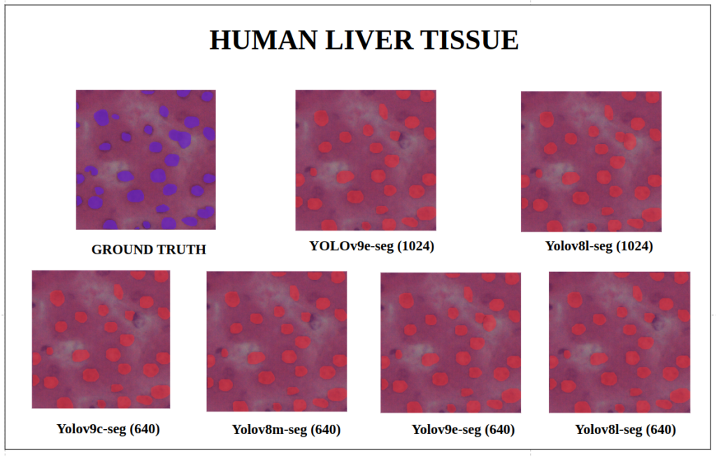
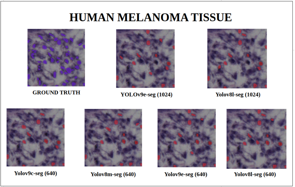
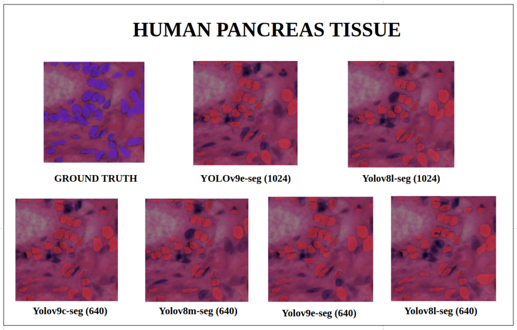
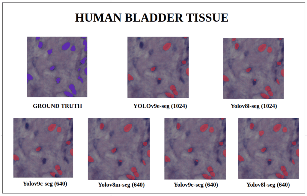
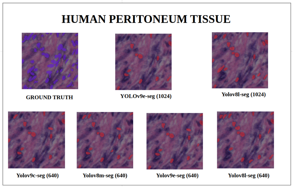
With a training configuration of  imgsz=1024 and inference conf=0.7, even though the YOLOv8l-seg ( 46M ) has comparatively very less parameters than YOLOv9e-seg ( 60.5 M ), in many instances YOLOv8l-seg outperformed.

On the other hand, comparing the YOLOv9c-seg ( 27.9M ) v/s YOLOv8m–seg ( 27.3M ),with imgsz=1024 overall, both performed nearly the same.

YOLOv9 Instance Segmentation Key Takeaways

Our experiment findings on fine-tuning YOLOv9 seg outlines as  follows :

• Both YOLOv9-seg and YOLOv8-seg models had good quantitative performance on instance segmentation tasks.
• From this article’s extensive set of experiments, it was observed that in some cases, even with comparatively fewer model parameters, the YOLOv8-seg models have a slight edge over YOLOv9-seg models on this Nuclei Cell Instance dataset.
• When the image size is increased to 1024, YOLOv9e-seg model performed worse than its relatively less parameter size models like YOLOv8l-seg, YOLOv8m-seg and same family YOLOv9c-seg.
  

Conclusion

In this article, we presented a comprehensive set of experiments on fine-tuning the YOLOv9 model, for instance segmentation tasks, emphasizing its potent utility in Medical Imaging.

Our study underscores the capacity of instance segmentation to deliver precise, object-level insights, which is crucial for applications ranging from cancer research to neurobiology and developmental biology.

References

[1]  NuInsSeg Kaggle Dataset

[2] Ultralytics Instance Segmentation Docs

[3]   Wang, Chien-Yao, Hong-Yuan Mark Liao, and I-Hau Yeh. “Designing network design strategies through gradient path analysis.” arXiv preprint arXiv:2211.04800 (2022).

[4]   Wang, Chien-Yao, I-Hau Yeh, and Hong-Yuan Mark Liao. “YOLOv9: Learning What You Want to Learn Using Programmable Gradient Information.” arXiv preprint arXiv:2402.13616 (2024).

[5]  YOLO Loss functions Part 1

[6]  YOLO Loss functions Part 2

[7] Fine-tuning YOLOv8 Instance Segmentation