Animal Pose Estimation: Fine-tuning YOLOv8 Pose Models

Animal pose estimation is an area of research within computer vision, a subfield of artificial intelligence, focused on automatically detecting and analyzing the postures and positions of animals in images or video footage. The goal is to determine the spatial arrangement of body parts, such as the head, limbs, and tail, for one or multiple animals. This technology has a wide array of applications, from studying animal behavior and biomechanics to wildlife conservation and monitoring.

In this blog post, we will specifically deal with keypoints estimation of dogs and show you how to fine-tune the very popular YOLOv8 pose models from Ultralytics.

Fine-tuning pose models for animal keypoints can be challenging and requires fine-tuning several hyperparameters. Luckily, YOLOv8 offers customization of quite a few of these hyperparameters during model fine-tuning. Precisely, we will fine-tune the following YOLOv8 pose models:

• YOLOv8m (medium)
• YOLOv8l (large)

Also, check out our in-depth human pose analysis by comparing inference results between YOLOv7 and MediaPipe pose models.

1. Stanford Dogs Dataset for Animal Pose Estimation
2. Dataset Anomalies for Animal Pose Estimation
   1. Handling Mismatched Ground Truth Annotations across Boxes and Keypoints for Animal Pose Estimation
3. Creating Annotations Consistent with YOLOv8 for Training and Validation Data
   1. Downloading Image Data and Keypoint Metadata
   2. Creating YOLO Train and Validation Directories for Animal Pose Estimation
   3. Creating Final YOLO Annotation Text Files
4. Hyperparameter Settings and Fine-Tuning for Animal Pose Estimation
   1. Training Configuration
   2. Data Configuration
   3. Fine-tuning and Training for Animal Pose Estimation
5. Evaluation of YOLOv8 on Animal Pose Estimation
6. Visualizations of Image Predictions on Animal Pose
7. Conclusion
8. References

YOLO Master Post –  Every Model Explained

Unlock the full story behind all the YOLO models’ evolutionary journey: Dive into our extensive pillar post, where we unravel the evolution from YOLOv1 to YOLO-NAS. This essential guide is packed with insights, comparisons, and a deeper understanding that you won’t find anywhere else.
Don’t miss out on this comprehensive resource, Mastering All Yolo Models for a richer, more informed perspective on the YOLO series.

Mastering All YOLO Models from YOLOv1 to YOLO-NAS: Papers Explained (2024)

Stanford Dogs Dataset for Animal Pose Estimation

For our animal pose estimation experiments, we will use the Stanford Dataset, which contains 120 breeds of dogs across 20,580 images. Besides, the dataset also contains the bounding box annotations for these images.

The keypoint annotations need to be downloaded from the StandfordExtra dataset by filling up a google form. The keypoint annotations are provided across 12,538 images for 20 keypoints of dog pose (3 for each leg, 2 for each ear, 2 for the tail, nose, and jaw).

The downloaded annotations will contain the following structure:

StanfordExtra_V12
├── StanfordExtra_v12.json
├── test_stanford_StanfordExtra_v12.npy
├── train_stanford_StanfordExtra_v12.npy
└── val_stanford_StanfordExtra_v12.npy

The train, validation, and test splits are provided as indices from the original StanfordExtra_v12.json data containing annotations for 6773, 4062, and 1703 images, respectively.

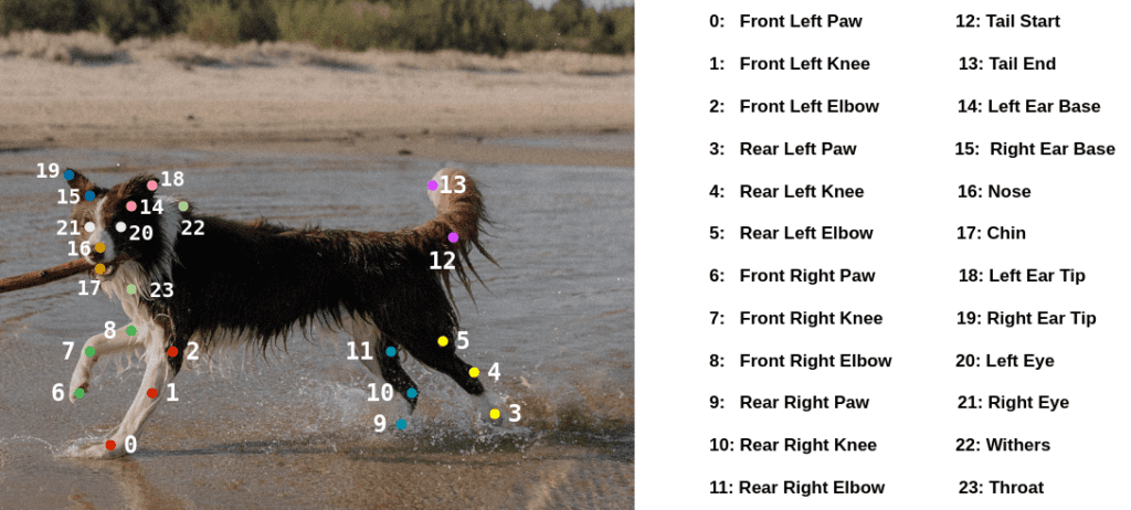
The authors have also provided keypoint metadata in the form of a CSV file containing the animal pose name, the color coding for each keypoint, etc. It, however, contains the info across 24 keypoints (1 for each eye, throat, and withers). The keypoints can be illustrated using the following image.

The annotations are present only for 20 of the 24 total keypoints. For the 4 left-out keypoints (2 for the eyes, throat, and wither), the coordinates are marked as 0s.

There is an additional boolean visibility flag that is associated with the 20 keypoints:

• 0: Not visible
• 1: Visible

Dataset Anomalies for Animal Pose Estimation

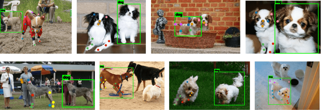
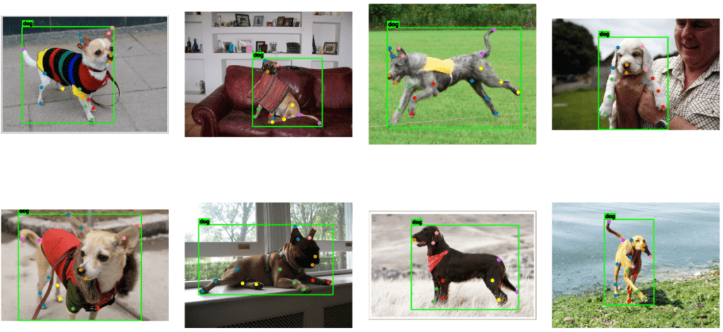
The ground truth annotations for the bounding boxes and keypoints are only available for single object instances. Besides, there are still quite a few incorrect annotations, as seen from the sample below.

The ground truth annotations for the bounding boxes and keypoints are only available for single object instances. Besides, there are still quite a few incorrect annotations, as seen from the sample below.

As you can see from the top leftmost image, the bounding box and the keypoints have been annotated for two different object instances. The same is reflected in the second and the fourth image in the 1st row (from left to right) and the first and the third image in the 2nd row.

Besides, the keypoints are also incorrectly annotated, as seen in the third image in the first row, where the jaw and the tip of the left ear are incorrectly annotated. The same is true for the first image in the second row, where the tip of the left ear has been mislabeled. Another instance of incorrect annotations has been manifested in the fourth image in the second row, where both ear tips are mislabelled.

As mentioned earlier, there are only single instance annotations for each image. Observe the second image (from the left) in the second row, where we only have annotations for the dog on the left, while there have been three instances of dogs.

Handling Mismatched Ground Truth Annotations across Boxes and Keypoints for Animal Pose Estimation

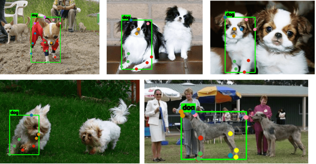
One intuitive way of handling mismatched box and keypoint annotations is to estimate a rectangle based on the given keypoints. This can be done using the cv2.boundingRect utility function to approximate a rectangle given a set of coordinates. Please pause for a moment and take a look at the samples below.

Although the bounding boxes are imperfect, handling mismatched bounding boxes and keypoint annotations can be inexpensive using the above approach. We can run a detection model such as YOLOv8 to obtain more accurate box annotations and then map the keypoints with the closest bounding box.

However, we shall stick to the annotations provided in the original JSON file for our experiments.

Click here to download the source code to this post

Creating Annotations Consistent with YOLOv8 for Training and Validation Data

Before we prepare our data, we need to be well-versed in the annotation format for keypoint detection accepted by YOLOv8 pose models from Ultralytics. The following points highlight the dataset format for fine-tuning Ultralytics’ YOLOv8 Pose models:

The dataset format used for training YOLO pose models is as follows:

1. One text file per image: Each image in the dataset has a corresponding text file with the same name as the image file and the .txt extension.
2. One row per object: Each row in the text file corresponds to one object instance in the image.
3. Object information per row: Each row contains the following information about the object instance:
   • Object class index: An integer representing the object’s class (e.g., 0 for person, 1 for car, etc.).
   • Object center coordinates: The x and y coordinates of the object’s center are normalized to 0 and 1.
   • Object width and height: The width and height of the object are normalized to be between 0 and 1.
   • Object width and height: The width and height of the object are normalized to be between 0 and 1.

Additionally, a visibility flag is associated with the keypoint coordinates. It can contain either of the three values:

•  0: Not labeled
•  1: Labelled but not visible
•  2: Labeled and visible.

The JSON annotations contain an additional boolean visibility flag and the keypoint coordinates discussed earlier. We will set the flags for all the visible keypoints to 2.

Keypoint annotations for fine-tuning pose models in Ultralytics correspond to the following syntax:

<class-index> <xc> <yc> <width> <height> <px1> <py1> <p1-visibility> ... <pxn> <pyn> <pn-visibility>

0 0.55991 0.503 0.76688 0.918 0.39143 0.91133 2.0 0.44227 0.72467 2.0 

The first item in the entry is the CLASS_ID, followed by the bounding box data (normalized x_center, y_center, width, height), and finally the normalized [x y] coordinates along with the visibility flags (i.e., 2 for both keypoints).

Downloading Image Data and Keypoint Metadata

Before we start with our data preparation, we need to download the image data first. Let us define a utility function that downloads and extracts the images.tar file containing the images. Besides, we shall also download the keypoint_definitions.csv containing the keypoint metadata, such as the animal pose name, color coding for each keypoint, etc., across all 24  keypoints.

def download_and_unzip(url, save_path):

    print("Downloading and extracting assets...", end="")
    file = requests.get(url)
    open(save_path, "wb").write(file.content)

    try:
        # Extract tarfile.
        if save_path.endswith(".tar"):
            with tarfile.open(save_path, "r") as tar:
                tar.extractall(os.path.split(save_path)[0])
            
        print("Done")
    except:
        print("Invalid file")

Let us now specify the images and the metadata URL and download them.

IMAGES_URL = r"http://vision.stanford.edu/aditya86/ImageNetDogs/images.tar"
IMAGES_DIR = "Images"
IMAGES_TAR_PATH = os.path.join(os.getcwd(), f"{IMAGES_DIR}.tar")

ANNS_METADATA_URL = r"https://github.com/benjiebob/StanfordExtra/raw/master/keypoint_definitions.csv"
ANNS_METADATA = "keypoint_definitions.csv"

# Download if dataset does not exists.
if not os.path.exists(IMAGES_DIR):
    download_and_unzip(IMAGES_URL, IMAGES_TAR_PATH)
    os.remove(IMAGES_TAR_PATH)

if not os.path.isfile(ANNS_METADATA):
    download_and_unzip(ANNS_METADATA_URL, ANNS_METADATA)

All the downloaded images are extracted to the Images  directory. It has the following directory structure:

Images/
├── n02085620-Chihuahua
│   ├── n02085620_10074.jpg
│   ├── n02085620_10131.jpg
│   └── ...
├── n02085782-Japanese_spaniel
│   ├── n02085782_1039.jpg
│   ├── n02085782_1058.jpg
│   └── n02085782_962.jpg
└── ...

It specifies the image files across all 120 categories of dogs.

Creating YOLO Train and Validation Directories for Animal Pose Estimation

Before we create the train and validation data for animal pose estimation, we need to have the annotation JSON file. The StanfordExtra_V12 directory houses the StanfordExtra_v12.json file along with the train, validation, and test splits.

StanfordExtra_V12
├── StanfordExtra_v12.json
├── test_stanford_StanfordExtra_v12.npy
├── train_stanford_StanfordExtra_v12.npy
└── val_stanford_StanfordExtra_v12.npy

Let us now read the annotation file.

ANN_PATH = "StanfordExtra_V12"
JSON_PATH = os.path.join(ANN_PATH, "StanfordExtra_v12.json")

with open(JSON_PATH) as file:
    json_data = json.load(file)

Each entry in the list json_data is a dictionary containing the image and annotation information. An example instance can be of the following:

{'img_path': 'n02091134-whippet/n02091134_3263.jpg',
 'img_width': 360,
 'img_height': 480,
 'img_bbox': [21, 55, 328, 422],
 'is_multiple_dogs': False,
 'joints': [[175.33333333333334, 453.3333333333333, 1],
  [260.0, 367.0, 1],
  [248.0, 296.6666666666667, 1],
  [337.6666666666667, 302.6666666666667, 1],
  [333.0, 265.0, 1],
  [329.3333333333333, 231.33333333333334, 1],
  [48.666666666666664, 415.0, 1],
  [167.0, 340.5, 1],
  [182.66666666666666, 280.3333333333333, 1],
  [0, 0, 0],
  [250.5, 253.0, 0],
  [277.0, 211.0, 0],
  [297.0, 200.5, 0],
  [0, 0, 0],
  [263.0, 117.0, 1],
  [193.66666666666666, 113.33333333333333, 1],
  [238.33333333333334, 182.0, 1],
  [231.66666666666666, 201.33333333333334, 1],
  [287.0, 69.61702127659575, 1],
  [187.36363636363637, 59.0, 1],
  [0, 0, 0],
  [0, 0, 0],
  [0, 0, 0],
  [0, 0, 0]],
 'seg': ...}

It has the following keys:

• img_path: The path to the image file.
• img_width: The image width.
• img_height: The image height.
• img_box: The bounding box annotation in [x_min, y_min, width, height] format.
• is_multiple_dogs: A boolean to denote the presence of a single or multiple instances of dogs.
• joints: A list of each 24 keypoint pixel coordinates (x, y), each associated with a visibility flag of 0 and 1.
• seg: Segmentation mask in running length encoding (RLE).

The files: train_stanford_StanfordExtra_v12.npy and test_stanford_StanfordExtra_v12.npy consist of the training and validation indices with respect to the original json_data list.
For simplicity, we shall use the test data for validation. The training and the test sets comprise 6773 and 1703 samples, respectively.

train_ids = np.load(os.path.join(ANN_PATH, 
                                 "train_stanford_StanfordExtra_v12.npy"))
val_ids = np.load(os.path.join(ANN_PATH, 
                               "test_stanford_StanfordExtra_v12.npy"))

We will now create the train and validation directories per YOLO. Specifically, it will have the following directory structure:

animal-pose-data
├── train
│   ├── images (6773 files)
│   └── labels (6773 files)
└── valid
    ├── images (1703 files)
    └── labels (1703 files)

Let us now initialise and create the directory paths for the training and validation data.

DATA_DIR = "animal-pose-data"

TRAIN_DIR         = f"train"
TRAIN_FOLDER_IMG    = f"images"
TRAIN_FOLDER_LABELS = f"labels"

TRAIN_IMG_PATH   = os.path.join(DATA_DIR, TRAIN_DIR, TRAIN_FOLDER_IMG)
TRAIN_LABEL_PATH = os.path.join(DATA_DIR, TRAIN_DIR, TRAIN_FOLDER_LABELS)

VALID_DIR           = f"valid"
VALID_FOLDER_IMG    = f"images"
VALID_FOLDER_LABELS = f"labels"

VALID_IMG_PATH   = os.path.join(DATA_DIR, VALID_DIR, VALID_FOLDER_IMG)
VALID_LABEL_PATH = os.path.join(DATA_DIR, VALID_DIR, VALID_FOLDER_LABELS)

os.makedirs(TRAIN_IMG_PATH, exist_ok=True)
os.makedirs(TRAIN_LABEL_PATH, exist_ok=True)
os.makedirs(VALID_IMG_PATH, exist_ok=True)
os.makedirs(VALID_LABEL_PATH, exist_ok=True)

Next, we will use train_ids and val_ids to gather the image and annotation data using json_data obtained earlier.

train_json_data = []
for train_id in train_ids:
    train_json_data.append(json_data[train_id])

val_json_data = []
for val_id in val_ids:
    val_json_data.append(json_data[val_id])

Now, we will copy the image files using the image paths from train_json_data and val_json_data to the corresponding images folder for the train and valid data created earlier.

for data in train_json_data:
    img_file = data["img_path"]
    filename = img_file.split("/")[-1]
    copyfile(os.path.join(IMAGES_DIR, img_file),
             os.path.join(TRAIN_IMG_PATH, filename))


for data in val_json_data:
    img_file = data["img_path"]
    filename = img_file.split("/")[-1]
    copyfile(os.path.join(IMAGES_DIR, img_file),
             os.path.join(VALID_IMG_PATH, filename))

Creating Final YOLO Annotation Text Files

Our final task for data preparation is to create the boxes and the keypoint annotations in accordance with Ultralytics’ YOLO. Since we will deal with a single class (i.e., dogs), we set the class index to 0.

CLASS_ID = 0

Given that the boxes and landmarks are in absolute coordinates, we need to normalize them in the range [0, 1] with respect to the image resolution.

The function create_yolo_boxes_kpts performs the following tasks:

• Modifies visibility indicators for keypoints (setting the visibilities for labeled keypoints to 2).
• Normalizes the coordinates of both bounding boxes and keypoints relative to the image dimensions.
• Converts bounding boxes to <xc> <yc> <width> <height> in normalized form.

def create_yolo_boxes_kpts(img_size, boxes, lm_kpts):

    IMG_W, IMG_H = img_size
    # Modify kpts with visibilities as 1s to 2s.
    vis_ones = np.where(lm_kpts[:, -1] == 1.)
    lm_kpts[vis_ones, -1] = 2.

    # Normalizing factor for bboxes and kpts.
    res_box_array = np.array([IMG_W, IMG_H, IMG_W, IMG_H])
    res_lm_array = np.array([IMG_W, IMG_H])

    # Normalize landmarks in the range [0,1].
    norm_kps_per_img = lm_kpts.copy()
    norm_kps_per_img[:, :-1]  = norm_kps_per_img[:, :-1] / res_lm_array

    # Normalize bboxes in the range [0,1].
    norm_bbox_per_img = boxes / res_box_array 

    # Create bboxes coordinates to YOLO.
    # x_c, y_c = x_min + bbox_w/2. , y_min + bbox_h/2.
    yolo_boxes = norm_bbox_per_img.copy()
    yolo_boxes[:2] = norm_bbox_per_img[:2] + norm_bbox_per_img[2:]/2.

    return yolo_boxes, norm_kps_per_img

The following are the input parameters for create_yolo_boxes_kpts:

• img_size: A tuple indicating the image dimensions (width, height).
• boxes: The bounding boxes in [xmin, ymin, width, height] format.
• lm_kpts: Landmark keypoints having shape [24, 3] (3 for [x, y, visibility]).

We will finally create the txt files for YOLO based on the train_json_data and val_json_data obtained earlier. The function create_yolo_txt_files creates the required .txt annotations in YOLO using the create_yolo_boxes_kpts utility function explained above.

def create_yolo_txt_files(json_data, LABEL_PATH):

    for data in json_data:
    
        IMAGE_ID = data["img_path"].split("/")[-1].split(".")[0]
    
        IMG_WIDTH, IMG_HEIGHT = data["img_width"], data["img_height"]
        
        landmark_kpts  = np.nan_to_num(np.array(data["joints"], dtype=np.float32))
        landmarks_bboxes = np.array(data["img_bbox"], dtype=np.float32)
        
        bboxes_yolo, kpts_yolo = create_yolo_boxes_kpts(
                                            (IMG_WIDTH, IMG_HEIGHT),
                                            landmarks_bboxes,
                                            landmark_kpts)
        
        TXT_FILE = IMAGE_ID+".txt" 
        
        with open(os.path.join(LABEL_PATH, TXT_FILE), "w") as f:
                
            x_c_norm, y_c_norm, box_width_norm, box_height_norm = round(bboxes_yolo[0],5),\
                                                                  round(bboxes_yolo[1],5),\
                                                                  round(bboxes_yolo[2],5),\
                                                                  round(bboxes_yolo[3],5),\
            
            kps_flattend = [round(ele,5) for ele in kpts_yolo.flatten().tolist()]
            line = f"{CLASS_ID} {x_c_norm} {y_c_norm} {box_width_norm} {box_height_norm} "
            line+= " ".join(map(str, kps_flattend))            
            f.write(line)

It accepts the following arguments:

• json_data: A list of dictionaries where each dictionary contains image metadata, including image dimensions, keypoints (joints), and bounding boxes (img_bbox).
• LABEL_PATH: The path where the text files will be saved.

Note: We have used nan_to_num from NumPy to convert keypoint coordinates with NaNs to 0s.

The following example shows one such instance where the keypoint coordinates are NaNs.

'joints': [[423.5, 224.75, 1.0],
  [285.0, 284.0, 1.0],
  [265.0, 232.0, 0.0],
  [nan, nan, 0.0],
  [137.0, 238.0, 0.0],
  [153.0, 221.0, 0.0],
  [111.0, 212.6, 1.0],
  [75.0, 270.0, 0.0],
  [nan, nan, 0.0],
  [100.0, 234.0, 1.0],
  [nan, nan, 0.0],
  [nan, nan, 0.0],
  [87.0, 224.0, 0.0],
  [79.0, 218.0, 0.0],
  [312.6666666666667, 156.5, 1.0],
  [172.0, 133.83333333333334, 1.0],
  [223.5, 264.0, 1.0],
  [215.5, 304.8333333333333, 1.0],
  [nan, nan, 0.0],
  [nan, nan, 0.0],
  [nan, nan, 0.0],
  [nan, nan, 0.0],
  [nan, nan, 0.0],
  [nan, nan, 0.0]]

We will now create the training and validation annotations.

create_yolo_txt_files(train_json_data, TRAIN_LABEL_PATH)
create_yolo_txt_files(val_json_data, VALID_LABEL_PATH)

Visualizing Data from YOLO Annotations

Once we have created our YOLO-compatible data, we can visualize a few ground truth samples to ensure that our conversion was correct.

Before visualizing the samples, we can map the hexadecimal color codings available with keypoint_definitions.csv to RGB values.

ann_meta_data = pd.read_csv("keypoint_definitions.csv")
COLORS = ann_meta_data["Hex colour"].values.tolist()

COLORS_RGB_MAP = []
for color in COLORS:
    R, G, B = int(color[:2], 16), int(color[2:4], 16), int(color[4:], 16)
    COLORS_RGB_MAP.append({color: (R,G,B)})

The draw_landmarks function is used to annotate the corresponding landmark points on the image using COLORS_RGB_MAP.

def draw_landmarks(image, landmarks):
    
    radius = 5
    # Check if image width is greater than 1000 px.
    # To improve visualization.
    if (image.shape[1] > 1000):
        radius = 8

    for idx, kpt_data in enumerate(landmarks):

        loc_x, loc_y = kpt_data[:2].astype("int").tolist()
        color_id = list(COLORS_RGB_MAP[int(kpt_data[-1])].values())[0]

        cv2.circle(image,
                   (loc_x, loc_y),
                   radius,
                   color=color_id[::-1],
                   thickness=-1,
                   lineType=cv2.LINE_AA)

    return image

The draw_boxes function is used to annotate the bounding boxes along with the confidence scores (if passed) on the image.

def draw_boxes(image, detections, class_name = "dog", score=None, color=(0,255,0)):

    font_size = 0.25 + 0.07 * min(image.shape[:2]) / 100
    font_size = max(font_size, 0.5)
    font_size = min(font_size, 0.8)
    text_offset = 3

    thickness = 2
    # Check if image width is greater than 1000 px.
    # To improve visualization.
    if (image.shape[1] > 1000):
        thickness = 10

    xmin, ymin, xmax, ymax = detections[:4].astype("int").tolist()
    conf = round(float(detections[-1]),2)
    cv2.rectangle(image, 
                  (xmin, ymin),
                  (xmax, ymax),
                  color=(0,255,0),
                  thickness=thickness,
                  lineType=cv2.LINE_AA)

    display_text = f"{class_name}"

    if score is not None:
        display_text+=f": {score:.2f}"

    (text_width, text_height), _ = cv2.getTextSize(display_text, 
                                                   cv2.FONT_HERSHEY_SIMPLEX,
                                                   font_size, 2)

    cv2.rectangle(image,
                      (xmin, ymin),
                      (xmin + text_width + text_offset, ymin - text_height - int(15 * font_size)),
                      color=color, thickness=-1)

    image = cv2.putText(
                    image,
                    display_text,
                    (xmin + text_offset, ymin - int(10 * font_size)),
                    cv2.FONT_HERSHEY_SIMPLEX,
                    font_size,
                    (0, 0, 0),
                    2, lineType=cv2.LINE_AA,
                )
    
    return image

We now have the utils to annotate landmarks and bounding boxes. However, we need the absolute coordinates (boxes and keypoints) to annotate them on images—the visualize_annotations utility plots annotations after converting them to absolute coordinates.

Recall that the bounding box coordinates and the keypoints were normalized in the range [0, 1]. However, to plot them, we need the absolute coordinates.

The conversion mapping from YOLO bboxes to [xmin, ymin, xmax, ymax] is pretty straightforward and can be obtained using the following set of equations:

Similarly, the keypoints can denormalized (to the absolute coordinates) using the following equations:

Here, the width and height are the box width and height, respectively, whereas W and H are the image width and height, respectively.

def visualize_annotations(image, box_data, keypoints_data):

    image = image.copy()

    shape_multiplier = np.array(image.shape[:2][::-1]) # (W, H).
    # Final absolute coordinates (xmin, ymin, xmax, ymax).
    denorm_boxes = np.zeros_like(box_data)

    # De-normalize center coordinates from YOLO to (xmin, ymin).
    denorm_boxes[:, :2] = (shape_multiplier/2.) * (2*box_data[:,:2] - box_data[:,2:])

    # De-normalize width and height from YOLO to (xmax, ymax).
    denorm_boxes[:, 2:] = denorm_boxes[:,:2] + box_data[:,2:]*shape_multiplier

    for boxes, kpts in zip(denorm_boxes, keypoints_data):
        # De-normalize landmark coordinates.
        kpts[:, :2]*= shape_multiplier        
        image = draw_boxes(image, boxes)
        image = draw_landmarks(image, kpts)

    return image

The following plot shows a few image samples with their corresponding ground truth annotation. The keypoint annotations are filtered based on their corresponding visibility flag.

Animal Pose Estimation: Hyperparameter Settings and Fine-Tuning

Ultralytics offers the following pose models pre-trained on the MS-COCO dataset consisting of 17 keypoints.

For our experiments, we shall use the YOLOv8m-pose and YOLOv8l-pose models.

Training Configuration

We shall define the training configuration for fine-tuning in the TrainingConfig class.

@dataclass(frozen=True)
class TrainingConfig:
    DATASET_YAML:   str = "animal-keypoints.yaml"
    MODEL:          str = "yolov8m-pose.pt"
    EPOCHS:         int = 100
    KPT_SHAPE:    tuple = (24,3)
    PROJECT:        str = "Animal_Keypoints"
    NAME:           str = f"{MODEL.split('.')[0]}_{EPOCHS}_epochs"
    CLASSES_DICT:  dict = field(default_factory = lambda:{0 : "dog"})

Observe the KPT_SHAPE (keypoint shape) parameter. 24 denotes the number of keypoints to be trained while 3 indicating the x-y coordinates and the `visibility` flag. 

Data Configuration

The DatasetConfig class takes in the various hyperparameters related to the data, such as the image size and batch size to be used while training, along with the various augmentation probabilities such as Mosaic, horizontal flip, etc.

@dataclass(frozen=True)
class DatasetConfig:
    IMAGE_SIZE:    int   = 640
    BATCH_SIZE:    int   = 16
    CLOSE_MOSAIC:  int   = 10
    MOSAIC:        float = 0.4
    FLIP_LR:       float = 0.0 # Turn off horizontal flip.

Next, we instantiate the TrainingConfig and DatasetConfig classes.

train_config = TrainingConfig()
data_config = DatasetConfig()

Before we start our training, we need to create a yaml containing the path to the images and label files. We also need to specify the class names, starting from index=0 and the keypoint shape.

We can also provide the flip_idx parameter if the key points are symmetric along a reference point or a set of reference points (for example, the set of keypoints for the nose can be used as reference points for a face).

For example, if we assume five keypoints of the facial landmark: [left eye, right eye, nose, left mouth, right mouth], and the original index is [0, 1, 2, 3, 4], then flip_idx is [1, 0, 2, 4, 3]. This is essential when the horizontal flip is used as data augmentation.

Note: We have turned off horizontal (LR flip) for our experiment.

current_dir = os.getcwd()

data_dict = dict(
                path      = os.path.join(current_dir, DATA_DIR),
                train     = os.path.join(TRAIN_DIR, TRAIN_FOLDER_IMG),
                val       = os.path.join(VALID_DIR, VALID_FOLDER_IMG),
                names     = train_config.CLASSES_DICT,
                kpt_shape = list(train_config.KPT_SHAPE),
               )

with open(train_config.DATASET_YAML, "w") as config_file:
    yaml.dump(data_dict, config_file)

Fine-tuning and Training for Animal Pose Estimation

We will finally perform training using the configurations defined above.

pose_model = model = YOLO(train_config.MODEL)

pose_model.train(data    = train_config.DATASET_YAML,
            epochs       = train_config.EPOCHS,
            imgsz        = data_config.IMAGE_SIZE,
            batch        = data_config.BATCH_SIZE,
            project      = train_config.PROJECT,
            name         = train_config.NAME,
            close_mosaic = data_config.CLOSE_MOSAIC,
            mosaic       = data_config.MOSAIC,
            fliplr       = data_config.FLIP_LR
           )

Evaluation of YOLOv8 on Animal Pose Estimation

Recall that in object detection, Intersection over Union (IoU) is essential for finding the similarity between two boxes and, hence, computing the Mean Average Precision Precision (mAP). Its analogous to keypoint estimation is Object Keypoint Similarity (OKS).

OKS is defined as:

where,

• d_i is the Euclidean distance between the ground truth and the predicted keypoint i
• k is the constant for keypoint i
• s is the scale of the ground truth object; s² hence becomes the object’s segmented area.
• v_i is the ground truth visibility flag for keypoint i
• δ(v_i > 0) is the Dirac-delta function which computes as 1 if the keypoint i is labeled, otherwise 0

Check out our recent article, where we have discussed Object Keypoint Similarity (OKS) in depth.

Using the configurations above, we obtain the following metrics for YOLOv8m:

• Box Metrics:
  • mAP@50: 0.991
  • map@50-95: 0.922
• Pose Metrics:
  • mAP@50: 0.937
  • map@50-95: 0.497

The plots below show the metrics for YOLOv8m.

The following are the metrics for YOLOv8l using the same hyperparameter settings used for training YOLOv8m:

• Box Metrics:
  • mAP@50: 0.992
  • map@50-95: 0.932
• Pose Metrics:
  • mAP@50: 0.941
  • map@50-95: 0.509

The following plots show the logs for YOLOv8l:

Observe the steep decline in the box, cls, dfl, and pose losses after epoch 90. This is precisely when the mosaic augmentation was turned off!
You can also take a look at the tensorboard training logs for YOLOv8m and YOLOv8l.

Visualizations of Image Predictions

The prepare_predictions function obtains the corresponding image’s predicted boxes, confidence scores, and keypoints. It accepts the following thresholds:

• BOX_IOU_THRESH: To filter out overlapping bounding boxes greater than this threshold.
• `BOX_CONF_THRESH`: To filter boxes with confidence scores falling below this threshold.
• KPT_CONF_THRESH: To filter keypoint coordinates with confidence scores falling below the threshold.

def prepare_predictions(
    image_dir_path,
    image_filename, 
    model,
    BOX_IOU_THRESH = 0.55,
    BOX_CONF_THRESH=0.30,
    KPT_CONF_THRESH=0.68):

    image_path = os.path.join(image_dir_path, image_filename)
    image = cv2.imread(image_path).copy()

    results = model.predict(image_path, conf=BOX_CONF_THRESH, iou=BOX_IOU_THRESH)[0].cpu()

    if not len(results.boxes.xyxy):
        return image

    # Get the predicted boxes, conf scores and keypoints.    
    pred_boxes = results.boxes.xyxy.numpy()
    pred_box_conf = results.boxes.conf.numpy()
    pred_kpts_xy = results.keypoints.xy.numpy()
    pred_kpts_conf = results.keypoints.conf.numpy()

    # Draw predicted bounding boxes, conf scores and keypoints on image.
    for boxes, score, kpts, confs in zip(pred_boxes, pred_box_conf, pred_kpts_xy, pred_kpts_conf):
        kpts_ids = np.where(confs > KPT_CONF_THRESH)[0]
        filter_kpts = kpts[kpts_ids]
        filter_kpts = np.concatenate([filter_kpts, np.expand_dims(kpts_ids, axis=-1)], axis=-1)
        image = draw_boxes(image, boxes, score=score)
        image = draw_landmarks(image, filter_kpts)

    return image

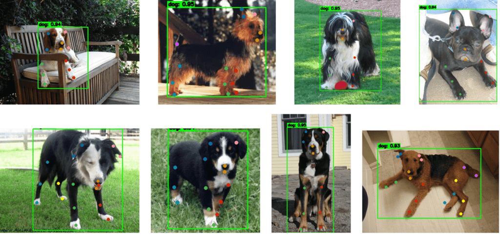
The following are the prediction samples from YOLOv8m pose model.

The plot below represents the visualization for YOLOv8l pose model.

Comparing the two inference samples, it seems that YOLOv8m performs slightly better than YOLOv8l even when the metrics for YOLOv8l are slightly higher.

We can confirm the same from the video sample below.

From the sample image and video inferences, we can observe that the models still have scope for improvements as the keypoints predictions, especially for the ear-tips and the tail, are not optimal. The predictions can be improved significantly by addressing the dataset anomalies we discussed earlier.

Conclusion

In this article, we have seen how to fine-tune YOLOv8 for animal pose estimation. We have also seen the presence of anomalies in our existing dataset, which has probably hindered model learning, as is evident from the sample inferences. 

The anomalies can be mitigated by correctly labeling the annotations, which could improve the metrics for the existing models.
Furthermore, we have also seen that YOLOv8 medium performs better in visualizations than YOLOv8 large, even though the metrics are slightly higher than YOLOv8m.

References

1. Stanford Dogs Dataset
2. StanfordExtra Repository
3. Ultralytics Pose Estimation Documentation
4. Ultralytics Pose Estimation Datasets Docs