The Intel-OpenVINO Toolkit provides many great functionalities for Deep-Learning model optimization, inference and deployment. Perhaps the most interesting and practical tool among them is the Deep-Learning (DL) workbench. Not only does model optimization, calibration, and quantization get easier, but the OpenVINO Deep Learning Workbench also makes the final model deployment-ready in a matter of minutes.
This post is the fourth in the OpenVINO series, which consists of the following posts:
- Introduction to OpenVINO Toolkit
- Post Training Quantization with OpenVino Toolkit
- Running OpenVino Models on Intel Integrated GPU
- Introduction to OpenVino Deep Learning Workbench
- Introduction to the OpenVINO Deep-Learning Workbench
- Installing the Deep-Learning Workbench through Docker
- AccuracyAwareQuantization Using DL Workbench
- Run Inference, Using INT8-Calibrated Tiny-YOLOv4 model
- Comparing Performance of FP32 With INT8 DefaultQuantization and AccuracyAwareQuantization Model
- COCO Evaluation Results
- Summary
After going through this final post in the OpenVINO series, you should be able to use the Deep-Learning workbench for your own projects, and optimize your Deep-Learning models as required.
Introduction to the OpenVINO Deep Learning Workbench
First, let’s understand what exactly is the DL workbench and why it’s important. It is a web-based application provided by the Intel OpenVINO toolkit that essentially runs in the browser. And it’s goal is to minimize the inference-to-deployment workflow timing for Deep-Learning models.
What makes it so useful?
- The DL workbench strongly integrates many of the optimization, quantization and deployment processes that OpenVINO supports, but are done manually.
- Its easy-to-use Graphical-User Interface lets you access almost everything, no need to bother what’s going on below the hood.
- You can not only import models and datasets, but also visualize and optimize these models.
- Even compare accuracies across various runs and parameters.
- Also, you can export the final model, which will be deployment-ready.
That’s not all, to learn what more you can do with the DL workbench, come let’s explore it well.
Functionalities and Components of the OpenVINO Deep Learning Workbench
Okay, so let’s study the functionalities and components that make the DL workbench so special.
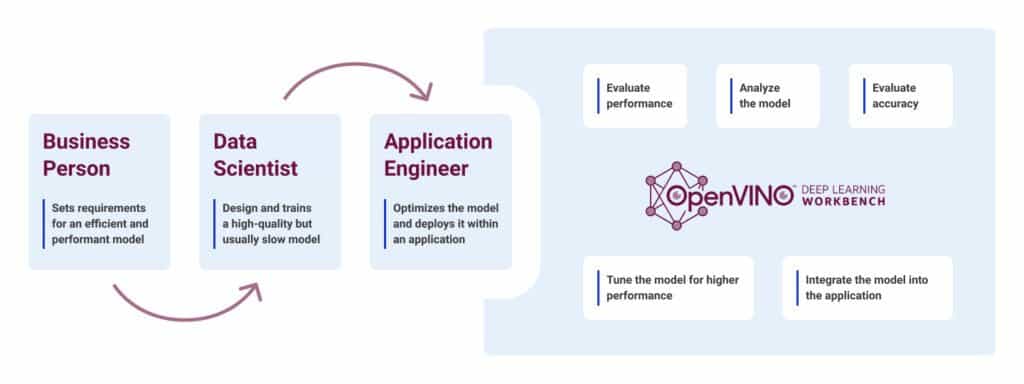
The general workflow of the DL workbench showing the basic functionalities
Have a look at the above image to understand the general workflow of the DL workbench and know the basic functionalities that come integrated with the following components:
- Model Evaluator
- Model Optimizer
- Model Quantization Tool
- Accuracy Checker
- Deployment Package Manager
Now, let’s go over them in a bit more detail.
1. Evaluating Model Performance
Like we already told you, the DL workbench allows you to import any model from its list of supported frameworks, which includes TensorFlow, ONNX, Caffe, MXNet and Kaldi. But did you know you can evaluate their performance too? Also, you can simply import a dataset of your choice, like the MS COCO or the PASCAL VOC dataset, and run an evaluation on them. Even if you do not have a standardized dataset at hand, you can always generate random data in the DL workbench itself.
Not only that, along with models from various frameworks, you can also import and evaluate models that are already in the OpenVINO-IR format.
2. Analyzing the Model
Furthermore, you get a great environment and visualization tools to analyze the architecture of your imported models.
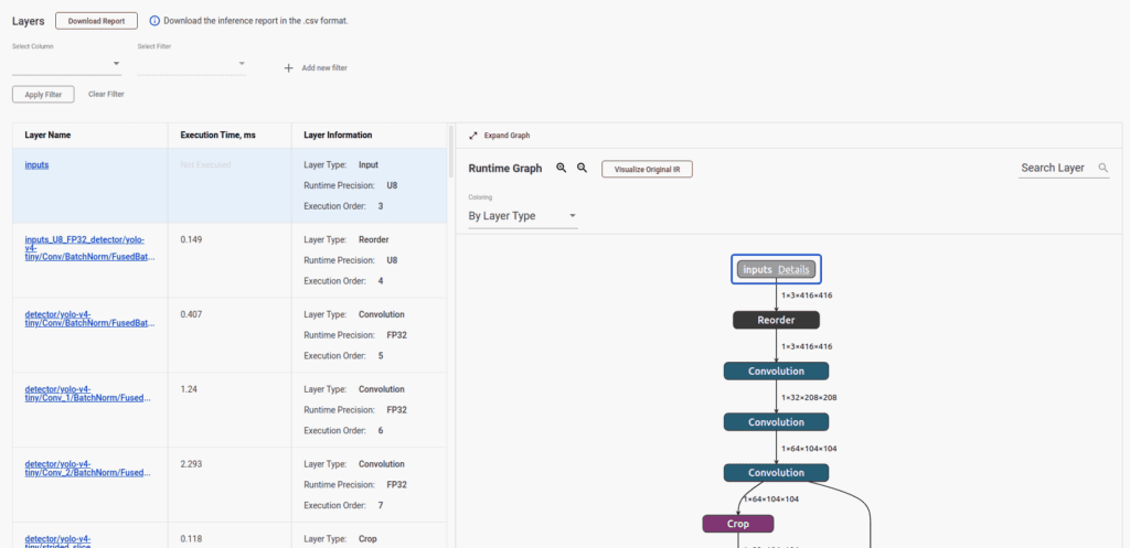
You can check each layer, each operation in the layers, and even how much time each layer took for every single operation. Then use these insights to further optimize your model and make it all the better.
3. Accuracy Evaluation
You can evaluate the accuracy of your imported models on various datasets, and this perhaps is the most important functionality available in the DL workbench.
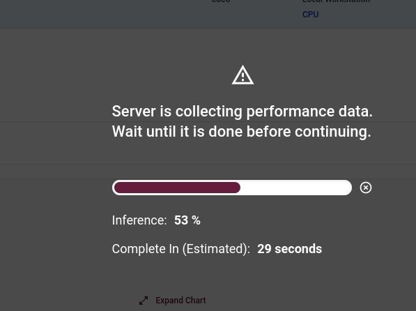
Simply choose the model, the target environment and the dataset on which to run the evaluation. And the workbench handles the rest. It will give you not only the accuracy, but also the FPS of the model for your chosen target environment. From there on, you decide whether to optimize it further or straightaway deploy.
4. Model Tuning and Quantization
Be it DefaultQuantization or AccuracyAwareQuantization, the process of model quantization becomes easier and hassle-free with the DL workbench.
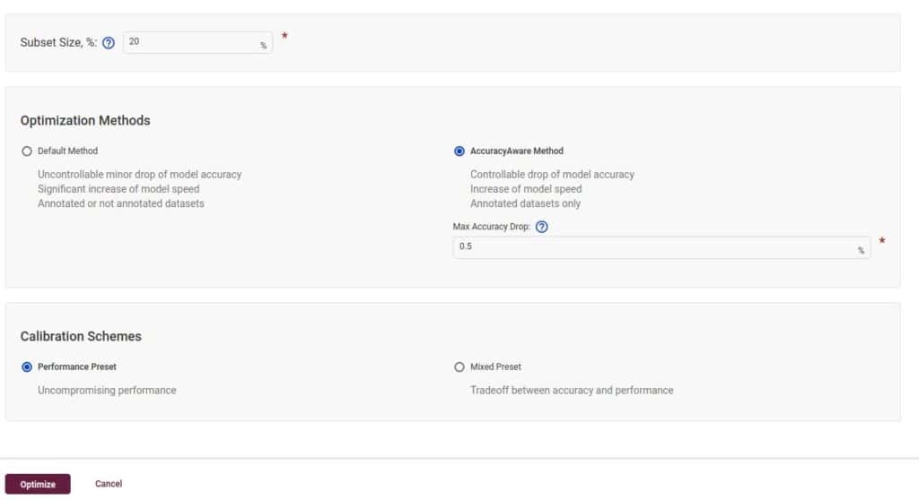
You will recall that in our previous Post Training Quantization post, we followed a series of manual steps to convert an FP32-Tiny YOLOv4 model into an INT8-precision model. Besides having to take care of each step and configuration file, we also had to ensure that each path and command was correct. With the DL workbench, you need not worry about any of these. Just provide the FP32 model, the dataset, and the desired accuracy. Within minutes, you will have an optimizer and a quantized model ready for use.
Note: Further down this post, you will learn how to quantize an FP32-Tiny YOLOv4 model into the INT8-precision format, using the AccuracyAwareQuantization with the DL workbench.
5. Integration and Deployment
Lastly, the DL workbench also provides a final-deployable model which you can just click and export. The exported, deployable package will contain:
- the optimized model
- all the configuration files
- the results of the various runs and experiments that you carry out
With all this information, you can easily zero in on the best possible way to deploy your model, and know exactly how it will perform. You can integrate it within an application, deploy it on the edge, or simply decide to run inference using the model.
Workflow of the Deep-Learning Workbench
The following diagram presents the workflow of the Deep-Learning workbench, illustrating all the steps, starting from model selection right up to model deployment:

As you can see, the general workflow consists of 7 steps. Let’s break these down into different components for greater clarity.
1. Model selection
You always start by selecting the model you want to optimize.
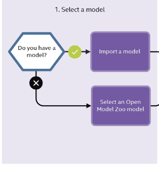
You are not constrained to choose a model from a specific framework, just ensure it comes from any of the OpenVINO-supported frameworks. You are even free to choose an OpenVINO-IR format model, provided you have already converted it using the Model Optimizer from any of the above frameworks.
2. Selecting the Target Environment
Next, select the target environment. This is important because the DL workbench will then optimize the model to run best on this particular hardware environment.
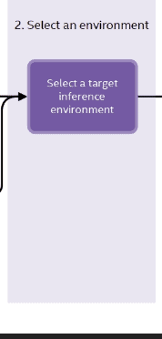
The target environment can be:
- a CPU
- the Intel Integrated GPU
- even VPUs like the Myriad X
In fact, you can even target a remote environment, which is not local to the system in which you are running the DL workbench.
3. Selecting the Dataset
Now that you’ve chosen the environment, select the dataset on which you want to run the evaluation and optimize the model.
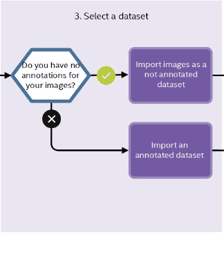
The DL workbench supports a number of datasets, including:
- Object-detection datasets like MS COCO, Pascal VOC
- Image-classification datasets like the ImageNet dataset
- Common Semantic Segmentation (CSS) dataset for semantic segmentation
- Common Super Resolution (CSR) dataset for super resolution, image inpainting and style transfer
4. Model Optimization
After model and dataset selection, optimize your model.
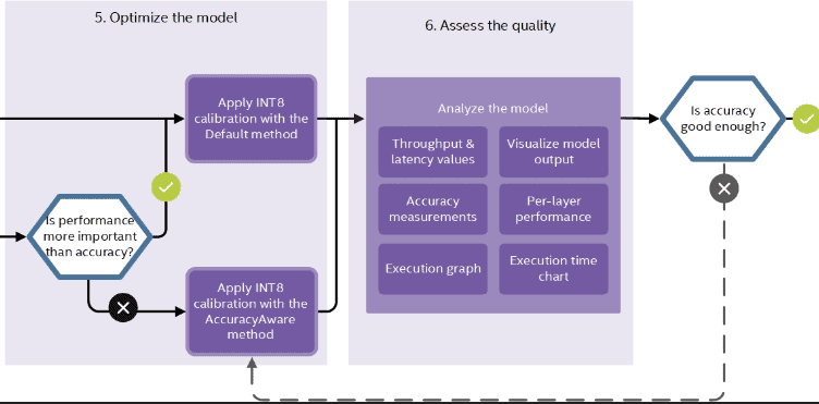
Apply quantization to convert the FP32 models into INT8-precision models. Also, assess the precision of your model, so that you know for sure it will perform well in the real-world.
5. Configure and Deploy
The final few steps will configure the model according to your requirements and deploy it.
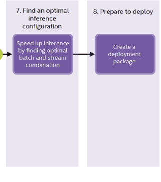
Experiment with different batch sizes and compare the throughput across different runs. When you get the desired tradeoff between speed and throughput:
- create the deployment package
- download it
- deploy it on an edge device
Don’t worry, we will be going through all these steps with you practically to ensure you get the required hands-on experience. We will convert the Tiny-YOLOv4 FP32 model into INT8 model, by applying AccuracyAwareQuantization, which itself will make most of these steps easy to grasp.
Installing Deep-Learning Workbench Through Docker
Only after you install the Deep-Learning workbench in your system can you use it for optimization.
The easiest way to install it is through the Docker Hub. First, install the Docker Engine, that being a necessary prerequisite. Please follow the instructions given here to install the Docker Engine on Ubuntu.
Now, follow these steps to install the DL workbench through Docker Hub on Linux (Ubuntu 20.04):
1. Go inside the workbench Folder in the OpenVINO Installation Directory
cd /opt/intel/openvino_2021.3.394/deployment_tools/tools/workbench
2. Download the Workbench Starting Script
To start the DL workbench, you need to download the script. Give the following command to download the starting script for DL workbench, inside the current working directory.
wget https://raw.githubusercontent.com/openvinotoolkit/workbench_aux/master/start_workbench.sh
3. Enure the File is Executable
In many cases, execution permissions are disabled by default for security reasons. Execute the following command to ensure the script is executable.
chmod +x start_workbench.sh
4. Run the DL Workbench
Finally, start the DL workbench through the terminal. ./start_workbench.sh
You may need to wait for some time till the DL workbench is ready. After the script runs all the commands successfully, a prompt on the terminal informs you that the DL workbench is available on the local host at port 5665.
Open the link and you will see the following browser window:

With this, you have completed the installation of DL workbench. Now, let’s quantize the models.
AccuracyAwareQuantization Using Deep-Learning Workbench
The Deep-Learning workbench makes it really easy to quantize models from FP32-precision format to INT8 precision. In fact, it supports both DefaultQuantization and AccuracyAwareQuantization.
We already carried out DefaultQuantization in our Post Training Quantization post in this series. Here, we will use the DL workbench to apply AccuracyAwareQuantization to the TIny-YOLOv4 model. There are mainly two reasons for going this way:
- The DL workbench will handle most of the heavy lifting that you otherwise would have to do manually.
- As of now, the Tiny-YOLOv4 model is not fully supported by OpenVINO. So, using POT (Post Training Optimization Toolkit) to quantize the Tiny-YOLOv4 model from FP32 to INT8 will give error. You can however successfully complete this process using the DL workbench.
Even when using the DL workbench, there are a few caveats when it comes to applying AccuracyAwareQuantization to Tiny YOLOv4. One such issue is that the DL workbench will not give the accuracy of the quantized model or even the full-precision model due to partial support. The reasons will be clear as you carry out the process yourself.
Applying AccuracyAwareQuantization to Tiny YOLOv4, Using DL Workbench
Just follow these steps:
1. Start the DL Workbench
First, open the DL workbench, by following all the steps discussed in the installation section.
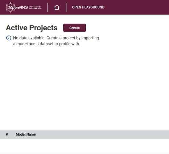
You will see the Create button at the top of the initial DL workbench window. Click on it.
2. Create Project
That takes you to the Create Project page, which should look similar to this:
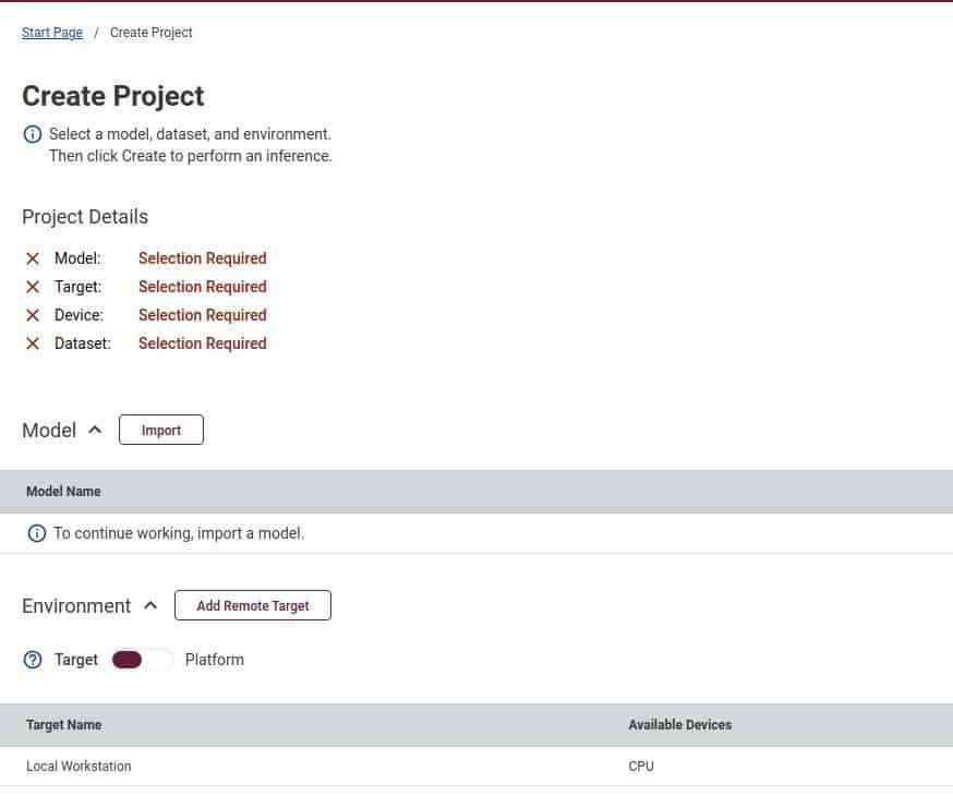
You need four things to successfully optimize a model, using the DL workbench:
- The Deep-Learning model
- The target environment
- The target device or hardware
- An evaluation dataset
Initially, all these options will be marked with red crosses (as in the above image), indicating that none of the requirements are met.
3. Import the Deep-Learning Model
Next, import the Deep-Learning model. For this example, we will be importing the Tiny-YOLOv4 FP32 model, which is already in the IR format. So no need to run it through the model optimizer. Simply, click on the Import button, which should take you to the following screen:
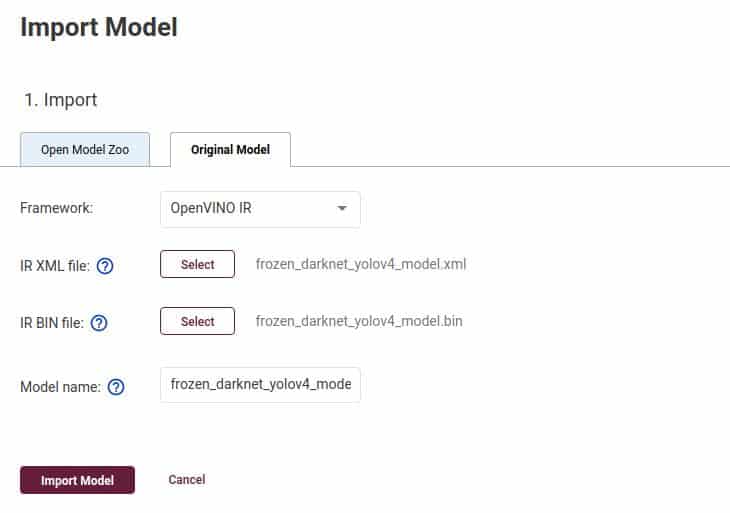
You will need both:
- The .
xmlfile containing the network topology - The .
binfile containing the model weights
Finally, click on the Import Model button. The model might take some time to upload to the DL-workbench environment.
4. Select the Target Environment and Hardware
Then you need to select the target environment and hardware.

For this example, we are using the Local Environment and the local CPU as our targets.
Note: The CPU used here is an i7 8670H laptop, with a base clock speed of 2.3 GHz and 16 GB of RAM.
When running on your local system, you should see your own CPU model and can choose accordingly.
5. Import the Evaluation Dataset
The final step before carrying out evaluation and optimization is to choose the evaluation dataset.
If you just needed to carry out the evaluation, you wouldn’t have to import any official dataset. Just creating a random dataset in the DL workbench would do. But here we need to quantize the model as well, so we will require a validation subset on which the quantized model can be evaluated.
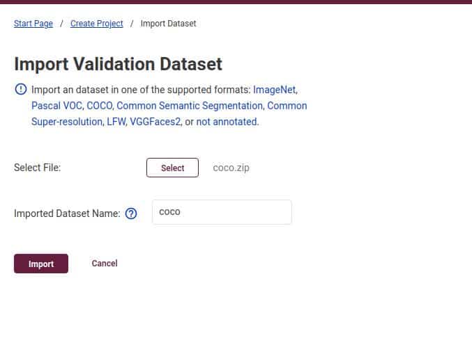
Here, we are importing the MS COCO 2017 validation dataset for evaluation purposes. This zip file contains 5000 validation images in total, along with their corresponding images. To download the dataset from the official website, click here.
After this, you should see a green tick mark across all the requirements.
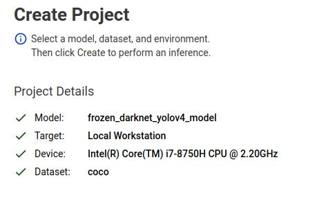
These are all the things you need to start the model evaluation/optimization. Next, click on the Create button on the browser window to start the process.
Initial Run Results
After this, run one initial evaluation on the entire validation dataset, using the full-precision model we selected above. Check out the results in the following image:

The above results are from the i7 CPU machine, as mentioned in the previous section. Your results may vary depending on the hardware. For the FP32 model, the initial is giving 27.6 FPS on average and latency of 35.17 milliseconds. It will be interesting to compare these results with the quantized model, after applying AccuracyAwareQuantization.
6. Optimize Performance
To start the AccuracyAwareQuantization:
- Click on the Perform tab on the current screen,
- Then click the Optimize Performance button. This should let you select the INT8-optimization method.

- Next, click the Optimize button.
7. Configure the Accuracy Settings and Select Dataset-Subset Size
Now you need to configure the accuracy settings. It is safe to leave the settings to default value initially. You should see a screen similar to this:

For the optimized configuration settings:
- The metric is mAP (mean Average Precision)
- The dataset is COCO with 80 classes
- Both IOU (Intersection Over Union) and NMS (Non Maximum Suppression) have 0.5 threshold
- The usage type is object detection, as we are using the Tiny YOLOv4 model
- The Model Type is set to Tiny YOLOv2
As you must have noticed by now, instead of v3 or v4, the Model Type is Tiny YOLOv2. Because the recent Tiny YOLO versions are not-fully supported by OpenVINO, we are bound to choose the Tiny YOLOv2 as the Model Type. Though this will not cause issues while quantizing the model, it will fail to give us any accuracy results. So, we will be checking the accuracy manually, by using the COCO evaluator to run evaluation manually on the entire COCO-validation set.
After completing the above settings, choose AccuracyAwareQuantization as the quantization method.

For this example, we have set the Max Accuracy Drop value to 0.5. This means, while doing INT8 calibration, if the accuracy drops below this specified threshold for any particular layer, then that layer will revert back to the original precision.
Also, take note of the dataset Subset Size. We are using just 20% of the 5000 images. So the calibration and evaluation will be done only on 1000 images. Selecting the whole dataset would have eaten up too much time, sometimes it takes hours to complete.
Finally, you can click on the Optimize button.
8. Check the Results
Let the calibration tool run the AccuracyAwareQuantization. It could take some time, depending on your hardware (CPU).
Here are the results from the i7 8th Generation 8670H CPU.

We got:
- 60 FPS, in terms of throughput
- The latency dropped to 17.66 milliseconds, after the INT8 calibration
This is a huge improvement compared to the 27 FPS and 35 milliseconds latency seen in the case of the full precision model.
We can also check the Precision Distribution in our calibrated model to ensure the model was actually converted to the INT8 format.

You can see that:
- More than 97% of the execution time was spent in the INT8 layers
- Around 2.7% of the time was spent in the FP32 layers
Okay, so this means most of the layers have been successfully converted to INT8 precision. Only a few layers reverted back to their original FP32-precision format, probably because they exceeded the accuracy-drop threshold of 0.5.
9. Export the Calibrated Model
The final step is to export your INT8-calibrated model so that you can run an inference with it.
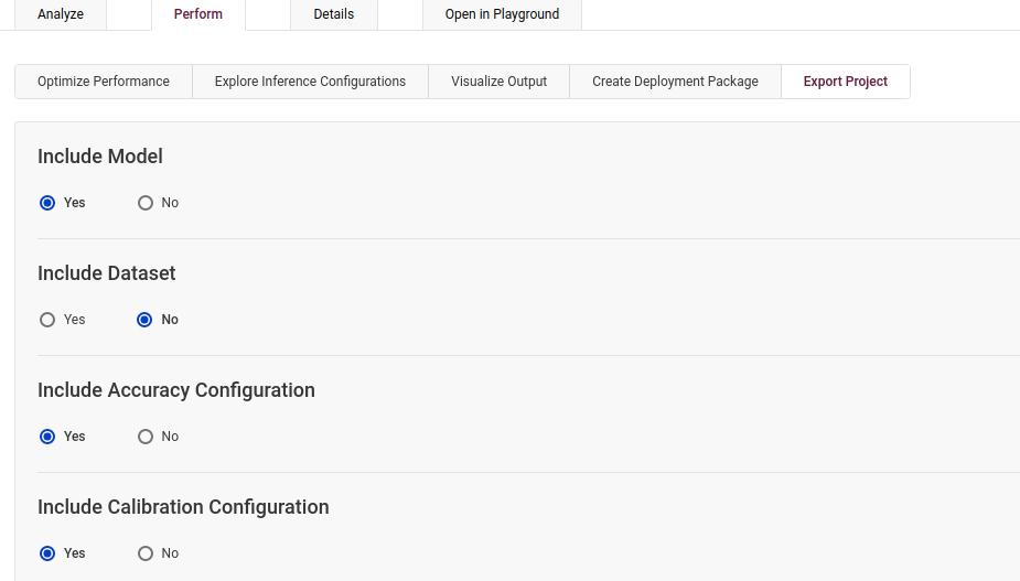
Go to the Export Project sub-tab on the Perform tab, choose the calibrated model, and click on the Export button. The downloaded file will contain the .xml as well as the .bin file.
Run Inference Using INT8-Calibrated Tiny-YOLOv4 Model
Now that we have obtained the INT8 models from the above steps, let’s try running inference on the following video.
To run inference, we use almost the same commands as in the previous posts in this series. The only difference being the path to the INT8-calibrated model. As the input video also remains the same, we can compare performance with the FP32 model.
python object_detection_demo.py --model frozen_darknet_yolov4_model.xml -at yolo -i video_1.mp4 -t 0.5 -o acc_aw_int8_default.mp4
For the above run:
- the average FPS is 30.3
- latency is 27.3 milliseconds
This is very close to what the INT8 model with DefaultQuantization gave in the Post Training Quantization post.
Now, check out the following video output:
The above results are really interesting. Not only are we getting throughput very similar to the Default Quantized INT8 model, but also the detections look exactly the same as the FP32 model. This means we are getting good speed and accuracy at the same time.
Let’s consider these graphs to double-check our speculations.
Comparing Performance of FP32 With INT8 DefaultQuantization and AccuracyAwareQuantization Model
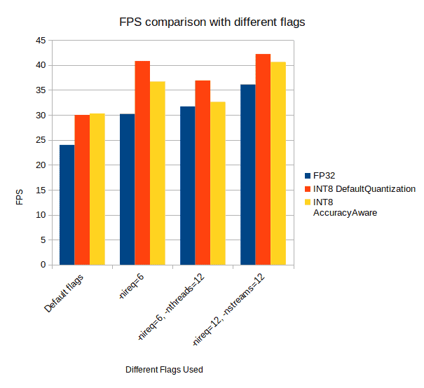
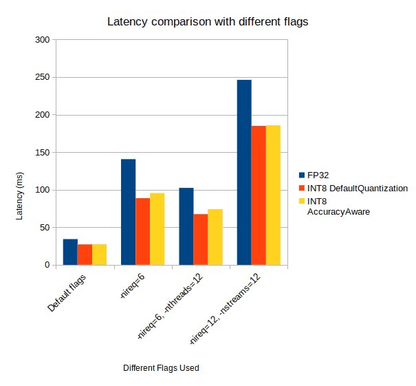
As you can see, the performance of INT8-DefaultQuantization Model and INT8-AccuracyAwareQuantization Model are running neck to neck. And in all the cases, the FPS is higher and latency is lower than the FP32 model.
Still, before we accept the AccuracyAwareQuantization-INT8 model as the final and best choice, it needs to pass one more test. So, let’s run the model evaluation on the entire COCO-evaluation dataset.
COCO Evaluation Results
We already discussed the steps to configure and install the COCO evaluator in second post of the series.
After running the COCO evaluator, the 5000 images from the MS COCO validation set, we get the following results.
 Average Precision  (AP) @[ IoU=0.50:0.95 | area=   all | maxDets=100 ] = 0.180
 Average Precision  (AP) @[ IoU=0.50      | area=   all | maxDets=100 ] = 0.332
 Average Precision  (AP) @[ IoU=0.75      | area=   all | maxDets=100 ] = 0.176
As you can see, the mAP is 0.180, which is:
- Even higher than the DefaultQuantization INT8 model that we saw in our Post-Training Quantization post.
- In fact, even higher than the FP32 model, which gave an mAP of 0.152.
This is quite amazing. Even the FPS in the above inference results almost matched that of the DefaultQuantization-INT8 model. It did fall short a bit, but the accuracy gain more than made up for that loss.
So, all in all, we can safely conclude that going with the AccuracyAwareQuantization Tiny YOLOv4 INT8 model turned out to be a good choice, both in terms of accuracy and speed.
Summary
In this post, you got introduced to the OpenVINO-Deep Learning Workbench and learned to use it for model evaluation and optimization.
- First, you explored all the different components needed for optimizing a Deep-earning model, using the DL workbench.
- Next, you went through all the steps necessary for applying AccuracyAwareQuantization to the Tiny-YOLOv4 INT8 model.
- After that, you studied several inference-comparison graphs, with FP32 and the DefaultQuantization model
- Finally, you concluded that the AccuracyAware-quantized model is the best choice to go with. The COCO evaluation results also proved it to be the best model.
Now you have all the tools that you need to optimize your Deep-Learning models for best performance and accuracy. We cannot wait to see what cool applications you come up with, using the techniques you learned. While building that next big thing, if there’s a wall or gap in your knowledge, don’t lose heart. Invest in our Deep Learning with PyTorch Course that takes care of basics as well as many advanced topics, and can make the next step easy for you.


100K+ Learners
Join Free OpenCV Bootcamp3 Hours of Learning