3D LiDAR object detection is a process that assists with identifying and localizing objects of interest in a 3-dimensional space. In autonomous systems and advanced spatial analysis, the evolution of object detection methodologies has been pivotal. Among these technologies, 3D LiDAR object detection is a transformative approach, offering unprecedented accuracy and depth in environmental perception.
In this comprehensive research article, we will extensively explore the implementation and training procedure for Keypoint Feature Pyramid Network (or) K-FPN using the KITTI 360 Vision dataset for autonomous driving with RGB cameras and 3D LiDAR fusion.
To see the results, you may SCROLL BELOW to the concluding part of the article or click here to see the experimental results right away.
PN: This research article is extensive, and if you feel overwhelmed by the intricate concepts, it is always better to start from the basics of ADAS. For this, it is advisible to explore 3D LiDAR visualization to understand the data distribution.
Intuition Behind Object Detection in a 3-Dimensional Space
3D object detection, at its core, is the process of identifying and localizing objects in three-dimensional space. Unlike 2D detection, which only considers the height and width on an image plane, 3D detection also incorporates depth, providing a complete spatial understanding. This is vital for applications such as autonomous driving, robotics, and augmented reality, where interaction with the environment is three-dimensional.
Human Depth Perception
The fundamental intuition behind 3D object detection stems from the way we, as humans, perceive depth. We infer the third dimension using cues such as shading, perspective, and parallax. In a similar vein, 3D detection algorithms leverage geometrical shapes, shadows, and the relative movement of points to discern depth.

Digital Depth Perception
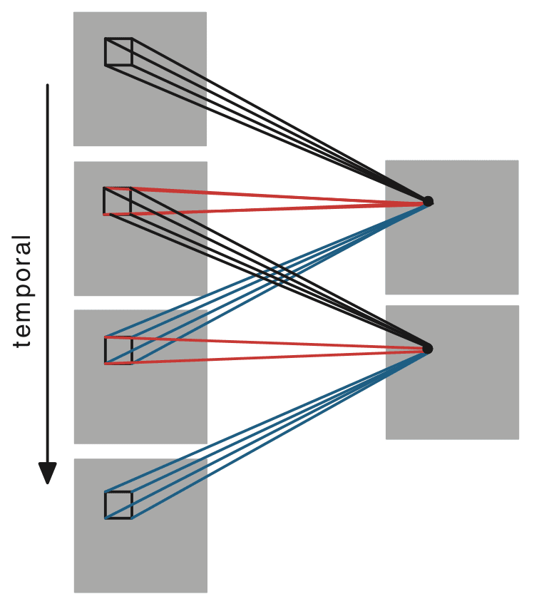
The first idea for a 3D-CNN was proposed by Shuiwang Ji et al., [1] in their research paper named ‘3D Convolutional Neural Networks for Human Action Recognition‘. Their model was able to extract features from both the spatial and temporal dimensions by performing 3D convolutions, thereby capturing the motion information encoded in multiple adjacent frames. This specific model generates multiple channels of information from the input frames, and the final feature representation combines information from all channels.
The representation of a 3D environment is typically through point clouds, which are sets of vertices in a three-dimensional coordinate system. These vertices are usually derived from structured light or LiDAR (Light Detection and Ranging) sensors. A critical aspect of 3D detection is the transformation of these point clouds into a format that can be processed to identify objects. This involves segmentation, where the point cloud is divided into clusters, each potentially representing an object. The clusters are then classified into known categories, such as cars, pedestrians, or other objects of interest.
The technical challenge here is significant due to the sparsity and variability of point cloud data. Unlike pixels in a 2D image, points in a 3D space do not have a uniform distribution, and their density can vary with distance from the sensor. Sophisticated algorithms such as PointNet and its successors (e.g., PointNet++) can directly process point clouds to learn features invariant to permutations and robust to occlusion and clutter.
Special Features of Detecting Objects in a 3D Point Cloud Environment
Detecting objects in a 3D point cloud environment introduces several special features not present in traditional 2D object detection:
- Depth Estimation: One of the most distinctive features is depth estimation, which allows the determination of an object’s distance from the sensor. Depth is directly measured in a point cloud, unlike in 2D images where it must be inferred.
- Volumetric Estimation: Algorithms can exploit the volumetric nature of data, considering objects’ actual shape and size. This is a departure from 2D bounding boxes, which only approximate the object’s footprint in the image plane.
- 6DoF (Six Degrees of Freedom) Object Pose: 3D detection algorithms not only localize objects but also determine their orientation in space, providing full 6DoF pose estimation (three for position and three for rotation).
- Scale Invariance: The detection process can be made invariant to the scale of the objects. This is particularly important for LiDAR-based systems, as objects may appear at various distances and thus at different scales.
- Temporal Continuity in Dynamic Environments: Advanced 3D object detection systems take advantage of temporal continuity in dynamic environments. By tracking the changes in point cloud data over time, they can predict the trajectories and velocities of moving objects.
Literature Review
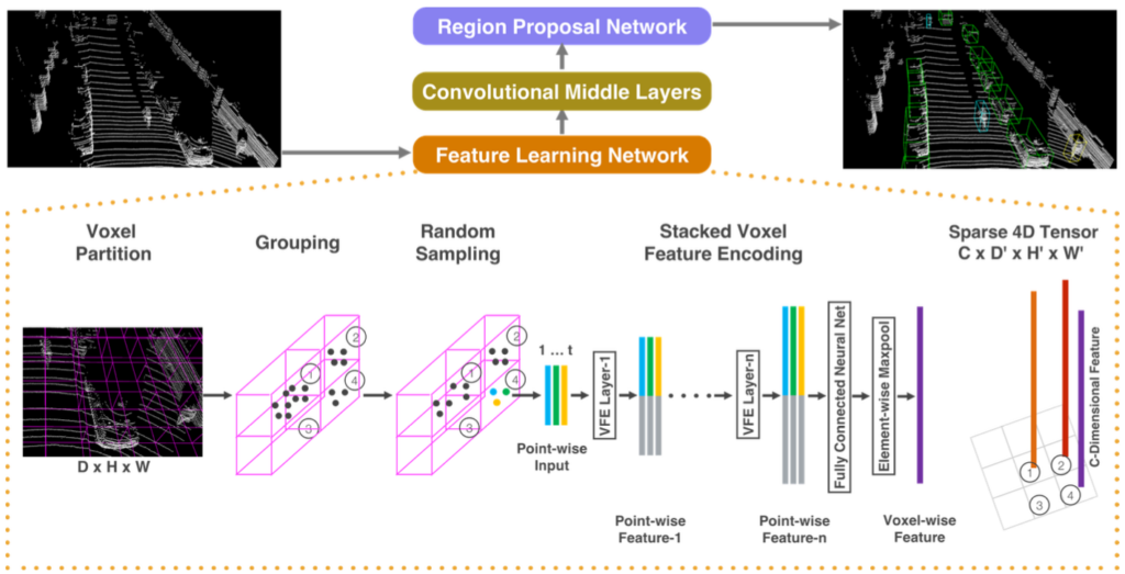
In their paper, Yin Zhou and Oncel Tuzel [2] proposed VoxelNet – an end-to-end learning for point cloud-based 3D object detection. VoxelNet innovatively partitions the point cloud into a structured 3D voxel grid and employs a unique voxel feature encoding layer to transform the points within each voxel into a comprehensive feature representation. This representation is seamlessly integrated with a Region Proposal Network (RPN) to generate object detections. Demonstrated on the KITTI benchmark for car detection, VoxelNet significantly surpasses existing LiDAR-based detection methods and exhibits a remarkable ability to learn distinct object representations, expanding its utility to detecting pedestrians and cyclists with promising results.
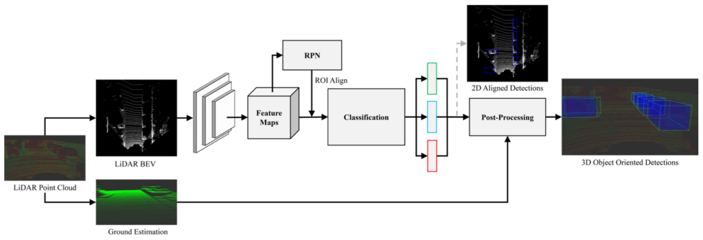
Jorge Beltrán et al., [3] introduced BirdNet – a 3D object detection framework from LiDAR information. Their method begins with an innovative cell encoding for bird’s eye view projection of laser data, followed by estimating object location and orientation using a convolutional neural network adapted from image processing techniques. The final stage involves post-processing to solidify 3D oriented detections. Validated on the KITTI dataset, their framework not only sets a new standard in the field but also exhibits versatility across different LiDAR systems, confirming its robustness in real-world traffic conditions.
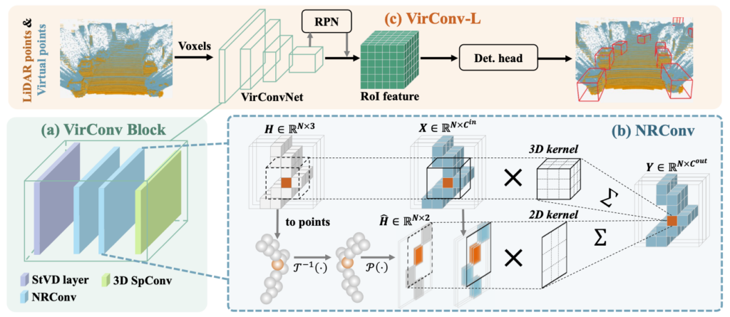
Hai Wu et al., [4] proposed VirConvNet, a novel and efficient backbone designed to enhance detection performance while managing computational load. Central to VirConvNet are two innovative components: StVD (Stochastic Voxel Discard), which strategically reduces redundant voxel computations, and NRConv (Noise-Resistant Submanifold Convolution), which robustly encodes voxel features by leveraging both 2D and 3D data. The authors showcase three variations of their pipeline: VirConv-L for efficiency, VirConv-T for precision, and VirConv-S for a semi-supervised approach. Impressively, their pipelines achieve top rankings on the KITTI car 3D detection leaderboard, with VirConv-S taking the lead and VirConv-L boasting a swift inference time.
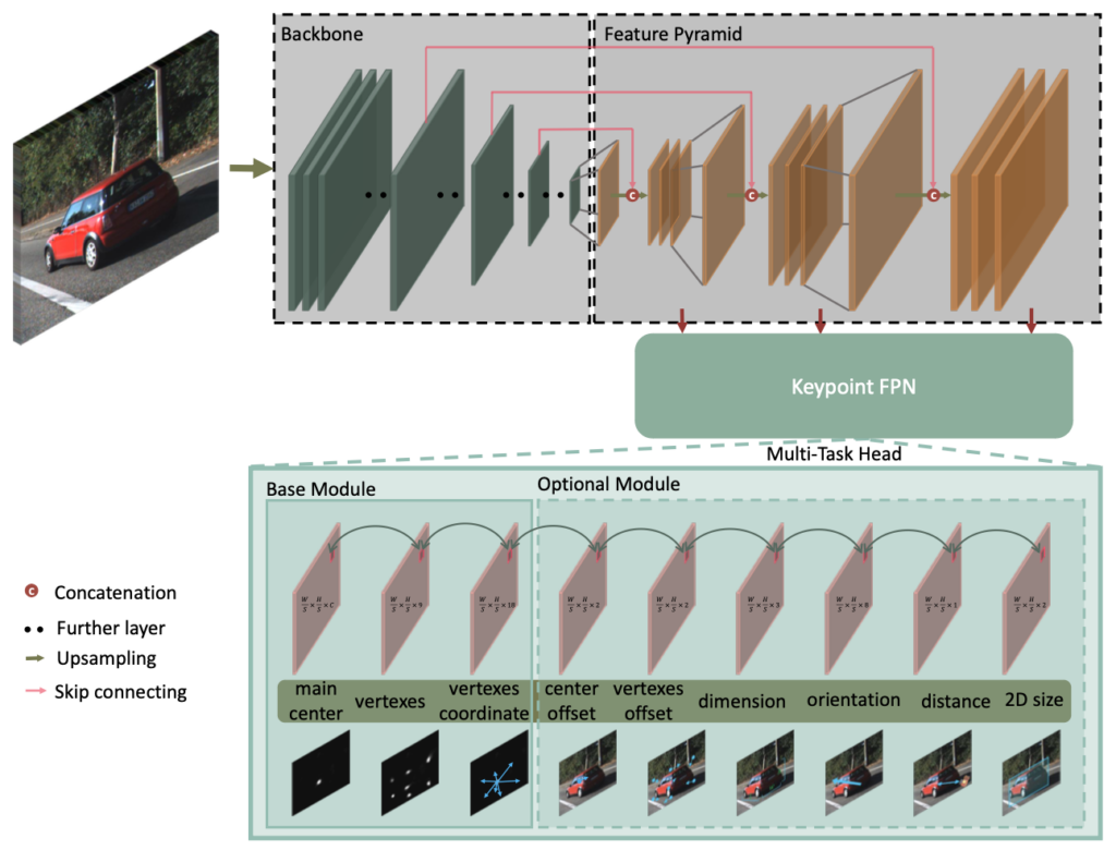
Peixuan Li et al., [5] developed a novel monocular 3D detection framework capable of efficient and accurate single-shot predictions. Moving away from traditional reliance on 2D bounding box constraints, their method innovatively predicts nine key points of a 3D bounding box from a monocular image, utilizing geometric relationships to accurately infer dimensions, location, and orientation in 3D space. This approach proves robust even with noisy keypoint estimations, facilitating rapid detection speeds with a compact architecture. Remarkably, their training regimen does not require external network dependencies or supervision data. The framework emerges as the first real-time system for monocular image 3D detection, setting a new benchmark in performance on the KITTI dataset.
Dataset Visualization for 3D LiDAR Object Detection
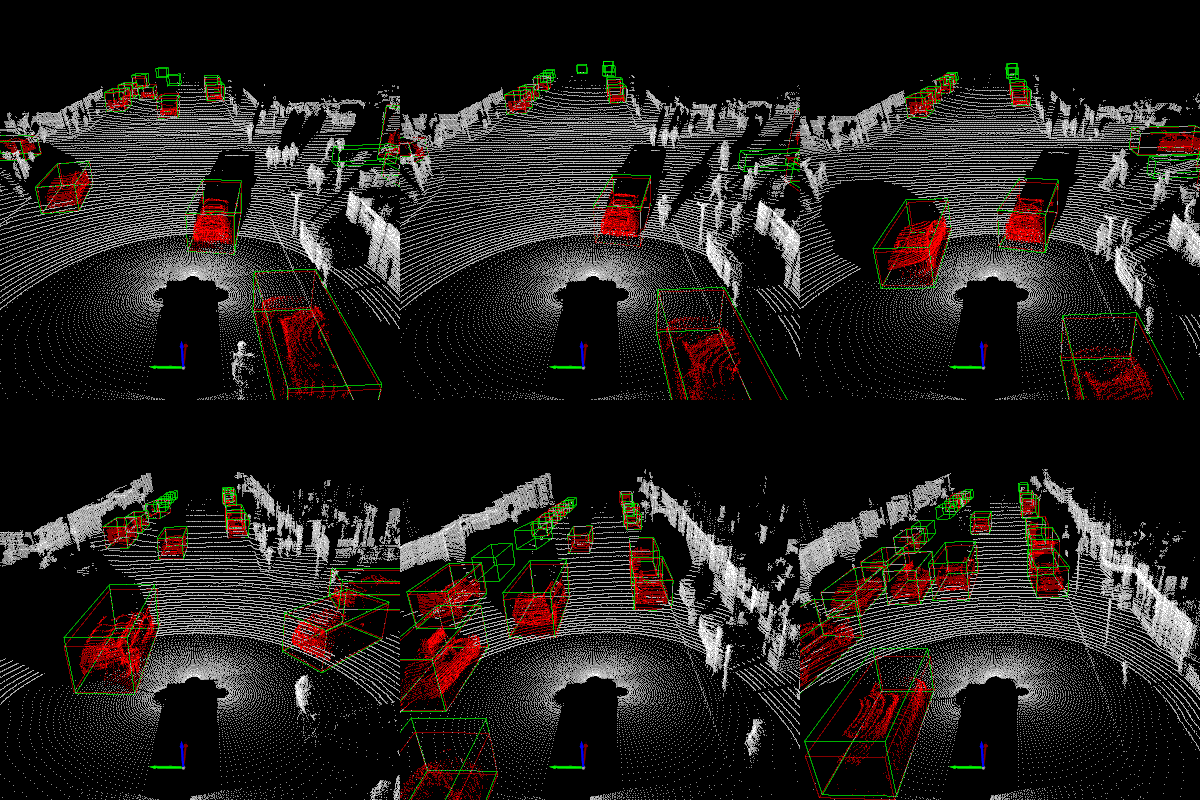
In this research article, we will use the KITTI 360 Vision dataset for the training procedure. This is a comparatively large dataset, and hence 3D LiDAR visualization is required for the EDA process. Here are a few visualization results from that experiment:
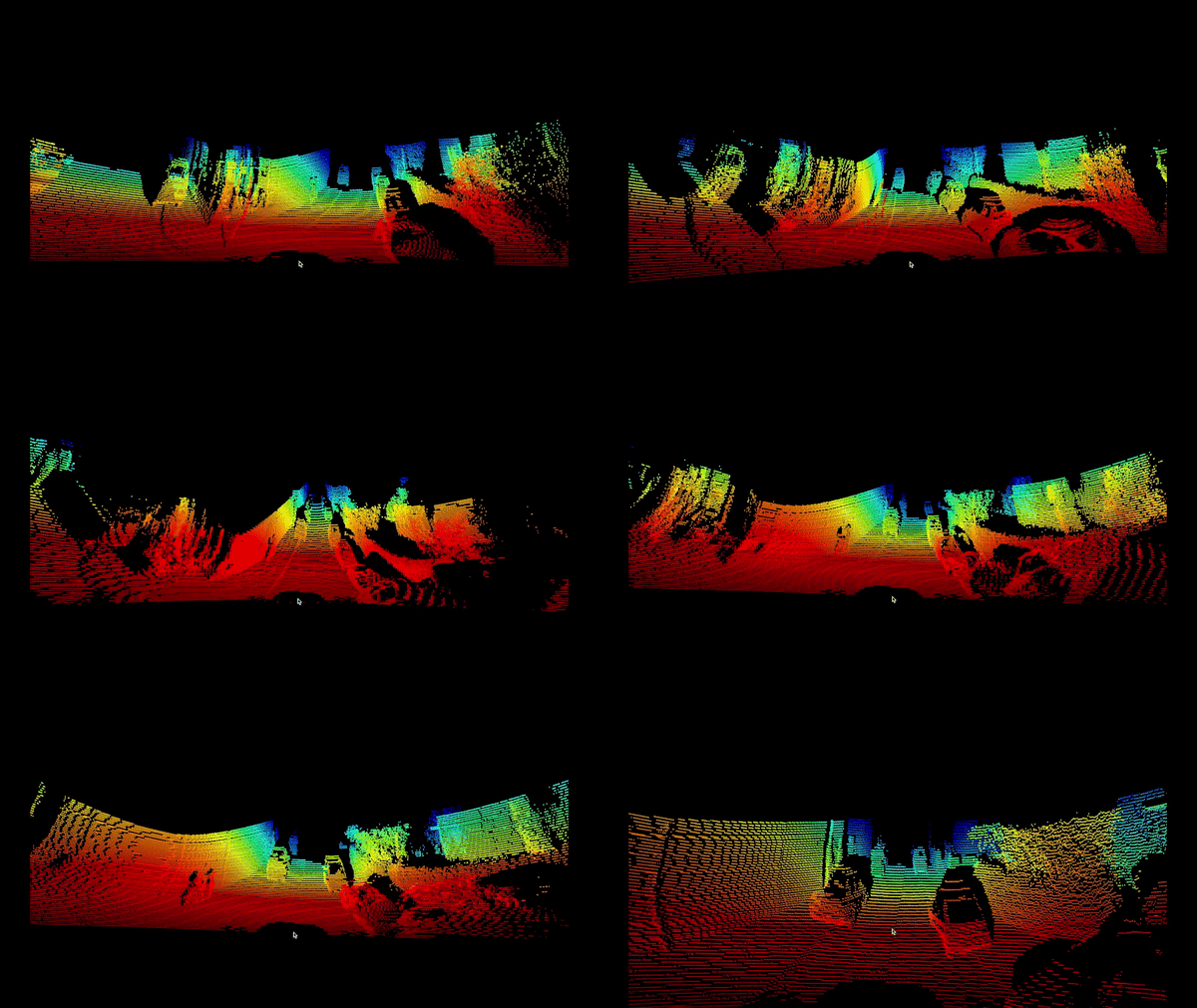
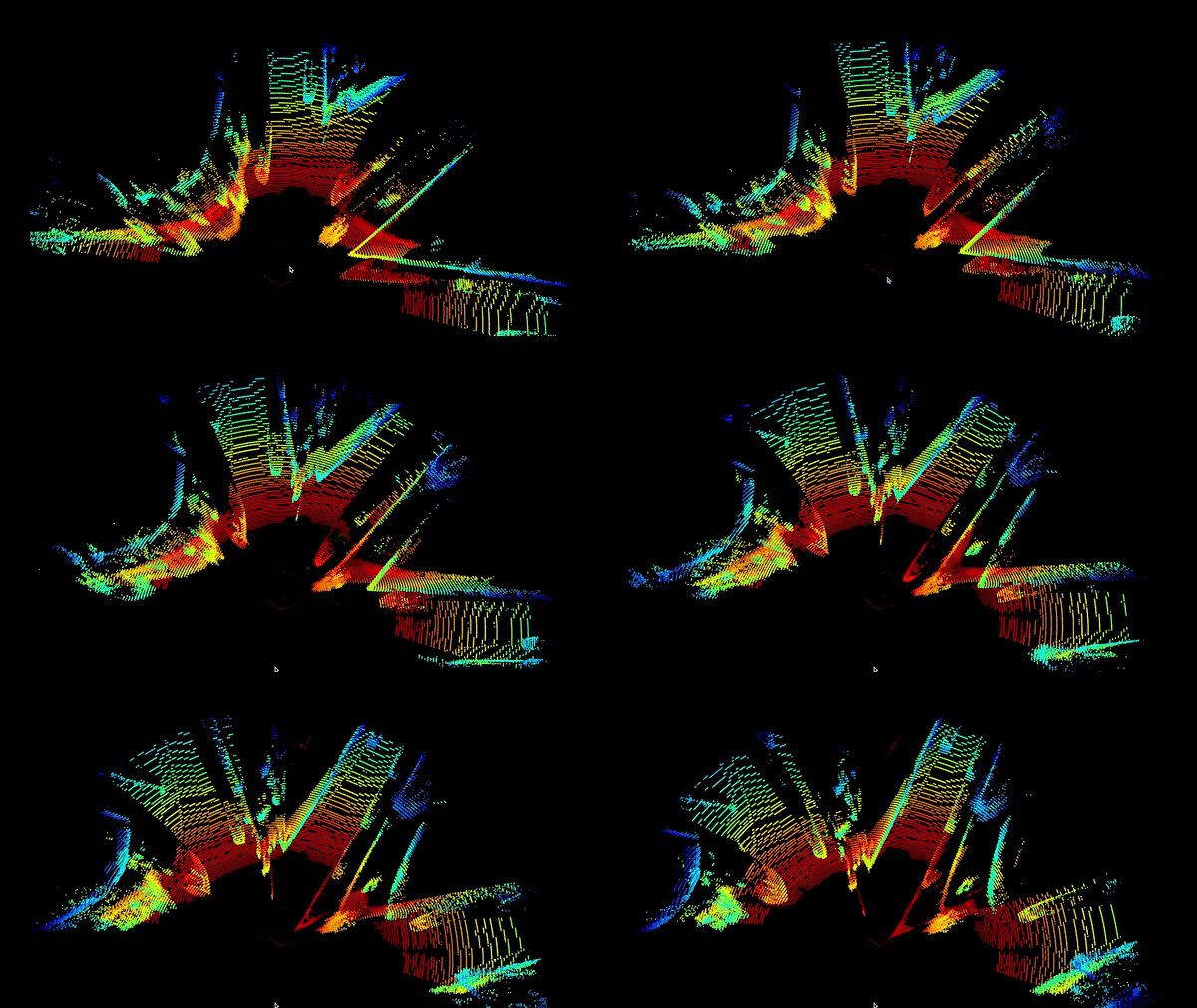
The visualizations shown in FIGURE 8 and FIGURE 9 highlight the 3-dimensional representation of the 3D LiDAR data from the sensor. However, it is also important to visualize 3D bounding boxes on the RGB camera stream, which is essential for developing advanced driver assistance systems. For this, you must first download the dataset and create a directory structure. Here are links to the specific files from the KITTI 360 Vision dataset:
- Velodyne Point Clouds – Laser Information (29GB)
- Training labels of Object Dataset (5MB)
- Camera calibration matrices of Object Dataset (16MB)
- Left color images of Object Dataset (12GB) – For Visualization
Now arrange the files such that the directory structure looks like this:
kitti
├── demo
│   └── calib.txt
├── gt_database
├── gt_database_mm
├── ImageSets
│   ├── train.txt
│   ├── test.txt
│   └── valid.txt
├── training
│   ├── image_2
│   ├── label_2
│   ├── calib
│   └── velodyne
├── testing
│   ├── image_2
│   ├── calib
│   └── velodyne
├── kitti_dbinfos_train.pkl
├── kitti_dbinfos_train_mm.pkl
├── kitti_infos_train.pkl
├── kitti_infos_trainval.pkl
├── kitti_infos_val.pkl
└── kitti_infos_test.pkl
Let’s take a minute and explore methods in the KittiDataset class defined in the kitti_dataset.py file within the codebase. You can download the code by SCROLLING DOWN to the code walkthrough section in this research article, or click here here.
This KittiDataset class is a custom dataset class suitable for loading and manipulating data from the KITTI 360 Vision dataset. This dataset class is tailored for different modes of operation such as training ('train'), validation ('val'), and testing ('test'), and is configured through a configs parameter that contains settings such as directory paths, input sizes, and the number of classes. This has been implemented in the kitti_dataset.py script within the data_process directory.
Here’s a breakdown of the class methods and their functionality:
def __init__(self, configs, mode='train', lidar_aug=None, hflip_prob=None, num_samples=None):
        self.dataset_dir = configs.dataset_dir
        self.input_size = configs.input_size
        self.hm_size = configs.hm_size

        self.num_classes = configs.num_classes
        self.max_objects = configs.max_objects

        assert mode in ['train', 'val', 'test'], 'Invalid mode: {}'.format(mode)
        self.mode = mode
        self.is_test = (self.mode == 'test')
        sub_folder = 'testing' if self.is_test else 'training'

        self.lidar_aug = lidar_aug
        self.hflip_prob = hflip_prob

        self.image_dir = os.path.join(self.dataset_dir, sub_folder, "image_2")
        self.lidar_dir = os.path.join(self.dataset_dir, sub_folder, "velodyne")
        self.calib_dir = os.path.join(self.dataset_dir, sub_folder, "calib")
        self.label_dir = os.path.join(self.dataset_dir, sub_folder, "label_2")
        split_txt_path = os.path.join(self.dataset_dir, 'ImageSets', '{}.txt'.format(mode))
        self.sample_id_list = [int(x.strip()) for x in open(split_txt_path).readlines()]

        if num_samples is not None:
            self.sample_id_list = self.sample_id_list[:num_samples]
        self.num_samples = len(self.sample_id_list)
This initializer method sets up the dataset by initializing paths to the various data directories (images, LiDAR, calibration, and labels) and creates a list of sample IDs to be used based on the mode of operation. It can optionally apply LiDAR data augmentation (lidar_aug) and horizontal flipping (hflip_prob) for data augmentation. If num_samples is specified, the dataset will truncate its length accordingly.
    def __len__(self):
        return len(self.sample_id_list)
This method returns the number of samples in the dataset, allowing PyTorch’s DataLoader to iterate over the dataset correctly.
    def __getitem__(self, index):
        if self.is_test:
            return self.load_img_only(index)
        else:
            return self.load_img_with_targets(index)
This method retrieves a single data point from the dataset. If the mode is ‘test’, it calls load_img_only, retrieving only the image data. For 'train' or 'val', it calls load_img_with_targets to get the image data and corresponding target labels.
    def load_img_only(self, index):
        """Load only image for the testing phase"""
        sample_id = int(self.sample_id_list[index])
        img_path, img_rgb = self.get_image(sample_id)
        lidarData = self.get_lidar(sample_id)
        lidarData = get_filtered_lidar(lidarData, cnf.boundary)
        bev_map = makeBEVMap(lidarData, cnf.boundary)
        bev_map = torch.from_numpy(bev_map)

        metadatas = {
            'img_path': img_path,
        }

        return metadatas, bev_map, img_rgb
This method is used during the testing phase to load only the image data and its associated metadata without any labels, as labels are not used during testing.
    def load_img_with_targets(self, index):
        """Load images and targets for the training and validation phase"""
        sample_id = int(self.sample_id_list[index])
        img_path = os.path.join(self.image_dir, '{:06d}.png'.format(sample_id))
        lidarData = self.get_lidar(sample_id)
        calib = self.get_calib(sample_id)
        labels, has_labels = self.get_label(sample_id)
        if has_labels:
            labels[:, 1:] = transformation.camera_to_lidar_box(labels[:, 1:], calib.V2C, calib.R0, calib.P2)

        if self.lidar_aug:
            lidarData, labels[:, 1:] = self.lidar_aug(lidarData, labels[:, 1:])

        lidarData, labels = get_filtered_lidar(lidarData, cnf.boundary, labels)

        bev_map = makeBEVMap(lidarData, cnf.boundary)
        bev_map = torch.from_numpy(bev_map)

        hflipped = False
        if np.random.random() < self.hflip_prob:
            hflipped = True
            # C, H, W
            bev_map = torch.flip(bev_map, [-1])

        targets = self.build_targets(labels, hflipped)

        metadatas = {
            'img_path': img_path,
            'hflipped': hflipped
        }

        return metadatas, bev_map, targets
This method loads the images and the target labels for training or validation. It applies any specified LiDAR augmentations and handles flipping the bird’s eye view (BEV) map if required. It also constructs the targets for object detection, including heatmaps, center offsets, dimensions, and orientations.
    def get_image(self, idx):
        img_path = os.path.join(self.image_dir, '{:06d}.png'.format(idx))
        img = cv2.cvtColor(cv2.imread(img_path), cv2.COLOR_BGR2RGB)

        return img_path, img
This method fetches the image file path and loads it using OpenCV, converting it from BGR to RGB format.
    def get_calib(self, idx):
        calib_file = os.path.join(self.calib_dir, '{:06d}.txt'.format(idx))
        # assert os.path.isfile(calib_file)
        return Calibration(calib_file)
This method retrieves the calibration data for the specified index, which is crucial for converting between camera and LiDAR coordinate systems.
    def get_lidar(self, idx):
        lidar_file = os.path.join(self.lidar_dir, '{:06d}.bin'.format(idx))
        # assert os.path.isfile(lidar_file)
        return np.fromfile(lidar_file, dtype=np.float32).reshape(-1, 4)
It loads the raw LiDAR data from a binary file and reshapes it into an N x 4 NumPy array where N is the number of points and the 4 represents the x, y, z coordinates and the reflection intensity.
    def get_label(self, idx):
        labels = []
        label_path = os.path.join(self.label_dir, '{:06d}.txt'.format(idx))
        for line in open(label_path, 'r'):
            line = line.rstrip()
            line_parts = line.split(' ')
            obj_name = line_parts[0]  # 'Car', 'Pedestrian', ...
            cat_id = int(cnf.CLASS_NAME_TO_ID[obj_name])
            if cat_id <= -99:  # ignore Tram and Misc
                continue
            truncated = int(float(line_parts[1]))  # truncated pixel ratio [0..1]
            occluded = int(line_parts[2])  # 0=visible, 1=partly occluded, 2=fully occluded, 3=unknown
            alpha = float(line_parts[3])  # object observation angle [-pi..pi]
            # xmin, ymin, xmax, ymax
            bbox = np.array([float(line_parts[4]), float(line_parts[5]), float(line_parts[6]), float(line_parts[7])])
            # height, width, length (h, w, l)
            h, w, l = float(line_parts[8]), float(line_parts[9]), float(line_parts[10])
            # location (x,y,z) in camera coord.
            x, y, z = float(line_parts[11]), float(line_parts[12]), float(line_parts[13])
            ry = float(line_parts[14])  # yaw angle (around Y-axis in camera coordinates) [-pi..pi]

            object_label = [cat_id, x, y, z, h, w, l, ry]
            labels.append(object_label)

        if len(labels) == 0:
            labels = np.zeros((1, 8), dtype=np.float32)
            has_labels = False
        else:
            labels = np.array(labels, dtype=np.float32)
            has_labels = True

        return labels, has_labels
This reads the object labels from the label files, including attributes such as object type, dimensions, and orientation.
    def build_targets(self, labels, hflipped):
        minX = cnf.boundary['minX']
        maxX = cnf.boundary['maxX']
        minY = cnf.boundary['minY']
        maxY = cnf.boundary['maxY']
        minZ = cnf.boundary['minZ']
        maxZ = cnf.boundary['maxZ']

        num_objects = min(len(labels), self.max_objects)
        hm_l, hm_w = self.hm_size

        hm_main_center = np.zeros((self.num_classes, hm_l, hm_w), dtype=np.float32)
        cen_offset = np.zeros((self.max_objects, 2), dtype=np.float32)
        direction = np.zeros((self.max_objects, 2), dtype=np.float32)
        z_coor = np.zeros((self.max_objects, 1), dtype=np.float32)
        dimension = np.zeros((self.max_objects, 3), dtype=np.float32)

        indices_center = np.zeros((self.max_objects), dtype=np.int64)
        obj_mask = np.zeros((self.max_objects), dtype=np.uint8)

        for k in range(num_objects):
            cls_id, x, y, z, h, w, l, yaw = labels[k]
            cls_id = int(cls_id)
            # Invert yaw angle
            yaw = -yaw
            if not ((minX <= x <= maxX) and (minY <= y <= maxY) and (minZ <= z <= maxZ)):
                continue
            if (h <= 0) or (w <= 0) or (l <= 0):
                continue

            bbox_l = l / cnf.bound_size_x * hm_l
            bbox_w = w / cnf.bound_size_y * hm_w
            radius = compute_radius((math.ceil(bbox_l), math.ceil(bbox_w)))
            radius = max(0, int(radius))

            center_y = (x - minX) / cnf.bound_size_x * hm_l  # x --> y (invert to 2D image space)
            center_x = (y - minY) / cnf.bound_size_y * hm_w  # y --> x
            center = np.array([center_x, center_y], dtype=np.float32)

            if hflipped:
                center[0] = hm_w - center[0] - 1

            center_int = center.astype(np.int32)
            if cls_id < 0:
                ignore_ids = [_ for _ in range(self.num_classes)] if cls_id == - 1 else [- cls_id - 2]
                # Consider to make mask ignore
                for cls_ig in ignore_ids:
                    gen_hm_radius(hm_main_center[cls_ig], center_int, radius)
                hm_main_center[ignore_ids, center_int[1], center_int[0]] = 0.9999
                continue

            # Generate heatmaps for main center
            gen_hm_radius(hm_main_center[cls_id], center, radius)
            # Index of the center
            indices_center[k] = center_int[1] * hm_w + center_int[0]

            # targets for center offset
            cen_offset[k] = center - center_int

            # targets for dimension
            dimension[k, 0] = h
            dimension[k, 1] = w
            dimension[k, 2] = l

            # targets for direction
            direction[k, 0] = math.sin(float(yaw))  # im
            direction[k, 1] = math.cos(float(yaw))  # re
            # im -->> -im
            if hflipped:
                direction[k, 0] = - direction[k, 0]

            # targets for depth
            z_coor[k] = z - minZ

            # Generate object masks
            obj_mask[k] = 1

        targets = {
            'hm_cen': hm_main_center,
            'cen_offset': cen_offset,
            'direction': direction,
            'z_coor': z_coor,
            'dim': dimension,
            'indices_center': indices_center,
            'obj_mask': obj_mask,
        }

        return targets
Based on the processed labels and augmentation information, this method builds the target variables for training the model. These include heatmaps for the object centers, offsets for the center points, object dimensions, orientation vectors, and a mask indicating the presence of objects.
    def draw_img_with_label(self, index):
        sample_id = int(self.sample_id_list[index])
        img_path, img_rgb = self.get_image(sample_id)
        lidarData = self.get_lidar(sample_id)
        calib = self.get_calib(sample_id)
        labels, has_labels = self.get_label(sample_id)
        if has_labels:
            labels[:, 1:] = transformation.camera_to_lidar_box(labels[:, 1:], calib.V2C, calib.R0, calib.P2)

        if self.lidar_aug:
            lidarData, labels[:, 1:] = self.lidar_aug(lidarData, labels[:, 1:])

        lidarData, labels = get_filtered_lidar(lidarData, cnf.boundary, labels)
        bev_map = makeBEVMap(lidarData, cnf.boundary)

        return bev_map, labels, img_rgb, img_path
In the end, this utility function is used to overlay labels on the BEV map for visualization purposes, which can be particularly helpful for understanding the data and debugging the dataset class.
Analysis of RGB POV Camera and 3D BEV LiDAR Point Cloud Simulations
Below are some visualizations generated by the KittiDataset class shown in the previous section.


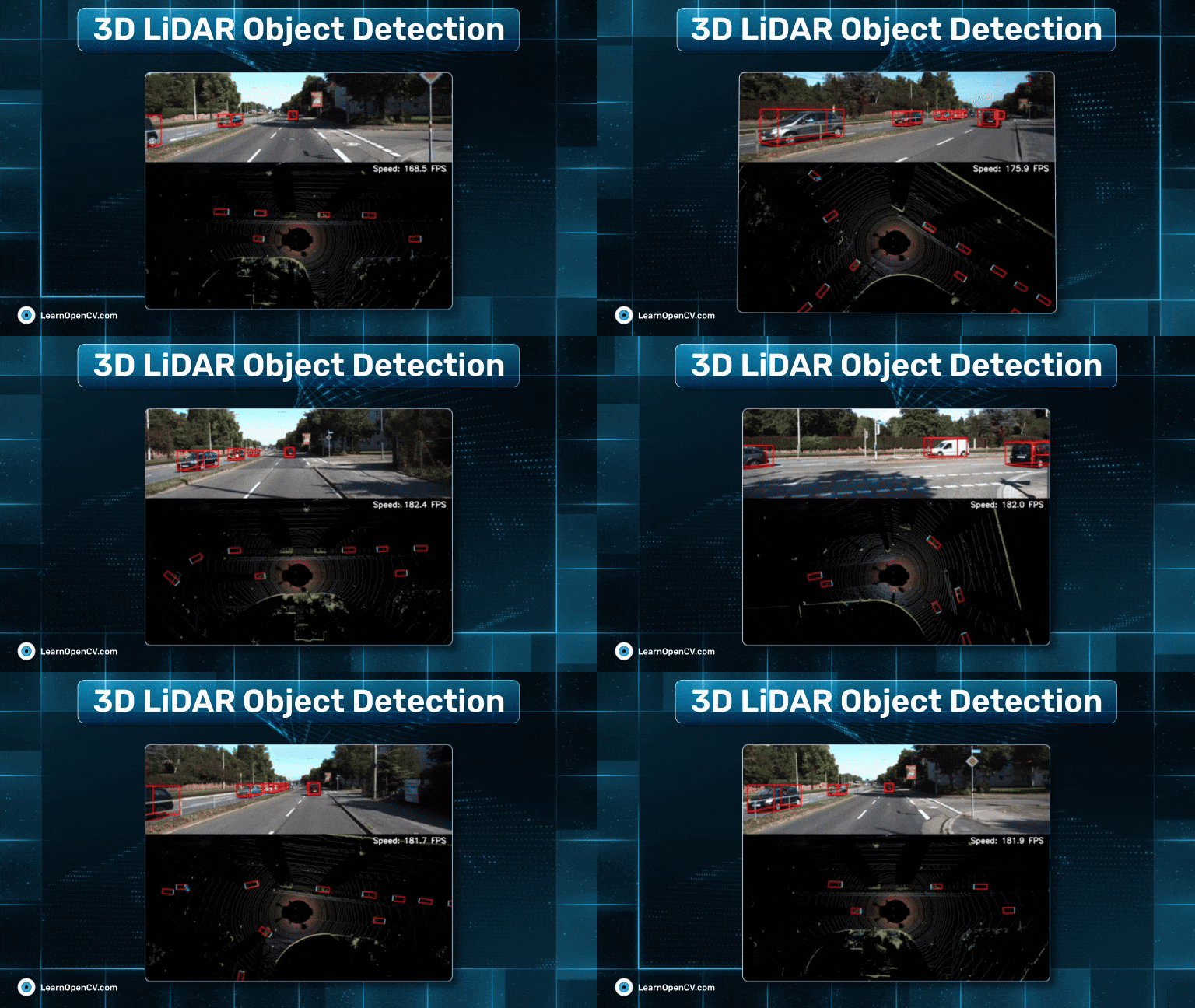
The top half of the image shows a standard POV camera view of a road scene, while the bottom half displays the corresponding bird’s eye view (BEV) from the 3D LiDAR data. Let’s take a closer look and analyze this visualization:
- RGB POV Camera View: Objects in the street-view such have been enclosed in the 3D bounding box, representing the object’s spatial extent in 3-dimensions: length, width and height.
- 3D BEV LiDAR View: The bottom image represents a BEV map constructed from the LiDAR points. In the BEV map, the world is viewed from a top view, the LiDAR data are projected onto a 2-dimensional plane. This projection helps understand the spatial layout and relationships between objects without the perspective distortion of a camera image. The red bounding box in the BEV corresponds to the 3D bounding box annotations from the camera view, flatted onto the 2D plane. It shows the location and orientation of the detected object relative to the vehicle’s position, which is often at the center of the concentric arcs. The concentric arcs represent the distance intervals from the 3D LiDAR sensor. They give a sense of scale and distance to the points and objects within the point cloud.
Keypoint Feature Pyramid Network Architecture
The Keypoint Feature Pyramid Network (KFPN), as detailed in the RTM3D research paper by Peixuan Li et al., [5], presents a sophisticated and nuanced approach to 3D object detection, particularly in the context of autonomous driving scenarios. This network architecture is tailored to process Bird’s Eye View (BEV) maps encoded from 3D LiDAR point clouds and output detailed object detections with seven degrees of freedom (7-DOF).
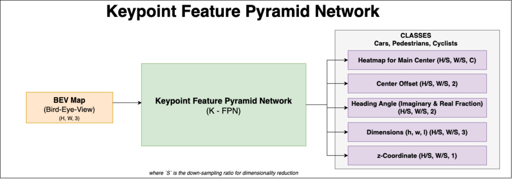
Let’s dive deeper into the technical architecture of this specific network:
Highlights
- Backbone Network: Utilizes ResNet-18 and DLA-34 backbones for initial image processing, applying a downsampling factor of
 for computational efficiency.
 - Upsampling and Feature Concatenation: Employs a series of bilinear interpolations and
 convolutions, enriching feature maps by concatenating them at each upsampling stage.
 - Keypoint Feature Pyramid: Adopts a novel approach for scale-invariant keypoint detection, resizing each scale feature map to a maximal scale for consistent keypoint analysis.
- Detection Head: Comprises a combination of fundamental and optional components, with heatmaps for the main center and vertex detection of 3D bounding boxes.
- Keypoint Association: Regresses local offsets for keypoint grouping and employs a Multi-Bin method for precise yaw angle estimation, enhancing 3D LiDAR object detection accuracy.
Backbone Network
The KFPN leverages two distinct structures for its backbone: ResNet-18 and DLA-34. These backbones are responsible for the initial processing of the single RGB input image, denoted as ![]() . The image undergoes downsampling by a factor of
. The image undergoes downsampling by a factor of ![]() , aligning with the standard practices in image classification networks where the maximum downsampling factor is ×32. The backbone’s role is crucial in feature extraction and reduction of computational complexity.
, aligning with the standard practices in image classification networks where the maximum downsampling factor is ×32. The backbone’s role is crucial in feature extraction and reduction of computational complexity.
Upsampling and Feature Concatenation
After the initial downsampling, the network employs a series of upsampling layers. This process involves three bilinear interpolations coupled with ![]() convolutional layers. Before each upsampling step, the network concatenates corresponding lower-level feature maps, followed by a
convolutional layers. Before each upsampling step, the network concatenates corresponding lower-level feature maps, followed by a ![]() convolutional layer to reduce channel dimensions. After these three upsampling layers, the output channels are 256, 128, and 64, respectively. This strategy ensures a rich feature representation encompassing both the input’s high-level and low-level details.
convolutional layer to reduce channel dimensions. After these three upsampling layers, the output channels are 256, 128, and 64, respectively. This strategy ensures a rich feature representation encompassing both the input’s high-level and low-level details.
Keypoint Feature Pyramid
In traditional Feature Pyramid Networks (FPN), multi-scale detection is common. However, for keypoint detection, where keypoints in the image do not vary significantly in size, the KFPN adopts a different approach. It proposes a novel keypoint feature pyramid to detect scale-invariant keypoints in point-wise space. This involves resizing each scale feature map back to the size of the maximal scale, generating feature maps ![]() , and then applying a softmax operation to derive the importance (weight) of each scale. The final scale-space score map,
, and then applying a softmax operation to derive the importance (weight) of each scale. The final scale-space score map, ![]() , is obtained through a linear weighted sum of these feature maps.
, is obtained through a linear weighted sum of these feature maps.
Detection Head
The detection head of KFPN comprises three fundamental components and six optional components. These components are designed to enhance the accuracy of 3D detection with minimal computational overhead. Inspired by CenterNet, the network employs a keypoint as the main center for connecting all features. The heatmap for this main center is defined as ![]() , where
, where ![]() denotes the number of object categories. The network also outputs a heatmap for nine perspective points projected by the vertices and center of the 3D bounding box, denoted as
denotes the number of object categories. The network also outputs a heatmap for nine perspective points projected by the vertices and center of the 3D bounding box, denoted as ![]() .
.
Keypoint Association and Additional Components
For associating key points of an object, the network regresses a local offset ![]() from the main center. This assists in grouping key points belonging to the same object. Additional components, such as the center and vertex offset, dimension of the 3D object, and orientation of the object, are included to provide more constraints and improve detection performance. The orientation is represented by the yaw angle
from the main center. This assists in grouping key points belonging to the same object. Additional components, such as the center and vertex offset, dimension of the 3D object, and orientation of the object, are included to provide more constraints and improve detection performance. The orientation is represented by the yaw angle ![]() , and the network utilizes a Multi-Bin method to regress the local orientation.
, and the network utilizes a Multi-Bin method to regress the local orientation.
Code Walkthrough – KFPN
Training Strategy
The training of the KFPN for 3D LiDAR object detection follows a strategy focusing on balancing the positive and negative samples. The focal loss is utilized to address this imbalance, a common approach in object detection networks to refine the learning process. This entire pipeline has been implemented in the train.py script. Let’s explore the functions that make up this training pipeline:
def main_worker(gpu_idx, configs):
    configs.gpu_idx = gpu_idx
    configs.device = torch.device('cpu' if configs.gpu_idx is None else 'cuda:{}'.format(configs.gpu_idx))

    if configs.distributed:
        if configs.dist_url == "env://" and configs.rank == -1:
            configs.rank = int(os.environ["RANK"])
        if configs.multiprocessing_distributed:
            # For multiprocessing distributed training, rank needs to be the
            # global rank among all the processes
            configs.rank = configs.rank * configs.ngpus_per_node + gpu_idx

        dist.init_process_group(backend=configs.dist_backend, init_method=configs.dist_url,
                                world_size=configs.world_size, rank=configs.rank)
        configs.subdivisions = int(64 / configs.batch_size / configs.ngpus_per_node)
    else:
        configs.subdivisions = int(64 / configs.batch_size)

    configs.is_master_node = (not configs.distributed) or (
            configs.distributed and (configs.rank % configs.ngpus_per_node == 0))

    if configs.is_master_node:
        logger = Logger(configs.logs_dir, configs.saved_fn)
        logger.info('>>> Created a new logger')
        logger.info('>>> configs: {}'.format(configs))
        tb_writer = SummaryWriter(log_dir=os.path.join(configs.logs_dir, 'tensorboard'))
    else:
        logger = None
        tb_writer = None

    # model
    model = create_model(configs)

    # load weight from a checkpoint
    if configs.pretrained_path is not None:
        assert os.path.isfile(configs.pretrained_path), "=> no checkpoint found at '{}'".format(configs.pretrained_path)
        model.load_state_dict(torch.load(configs.pretrained_path, map_location='cpu'))
        if logger is not None:
            logger.info('loaded pretrained model at {}'.format(configs.pretrained_path))

    # resume weights of model from a checkpoint
    if configs.resume_path is not None:
        assert os.path.isfile(configs.resume_path), "=> no checkpoint found at '{}'".format(configs.resume_path)
        model.load_state_dict(torch.load(configs.resume_path, map_location='cpu'))
        if logger is not None:
            logger.info('resume training model from checkpoint {}'.format(configs.resume_path))

    # Data Parallel
    model = make_data_parallel(model, configs)

    # Make sure to create optimizer after moving the model to cuda
    optimizer = create_optimizer(configs, model)
    lr_scheduler = create_lr_scheduler(optimizer, configs)
    configs.step_lr_in_epoch = False if configs.lr_type in ['multi_step', 'cosin', 'one_cycle'] else True

    # resume optimizer, lr_scheduler from a checkpoint
    if configs.resume_path is not None:
        utils_path = configs.resume_path.replace('Model_', 'Utils_')
        assert os.path.isfile(utils_path), "=> no checkpoint found at '{}'".format(utils_path)
        utils_state_dict = torch.load(utils_path, map_location='cuda:{}'.format(configs.gpu_idx))
        optimizer.load_state_dict(utils_state_dict['optimizer'])
        lr_scheduler.load_state_dict(utils_state_dict['lr_scheduler'])
        configs.start_epoch = utils_state_dict['epoch'] + 1

    if configs.is_master_node:
        num_parameters = get_num_parameters(model)
        logger.info('number of trained parameters of the model: {}'.format(num_parameters))

    if logger is not None:
        logger.info(">>> Loading dataset & getting dataloader...")
    # Create dataloader
    train_dataloader, train_sampler = create_train_dataloader(configs)
    if logger is not None:
        logger.info('number of batches in training set: {}'.format(len(train_dataloader)))

    if configs.evaluate:
        val_dataloader = create_val_dataloader(configs)
        val_loss = validate(val_dataloader, model, configs)
        print('val_loss: {:.4e}'.format(val_loss))
        return

    for epoch in range(configs.start_epoch, configs.num_epochs + 1):
        if logger is not None:
            logger.info('{}'.format('*-' * 40))
            logger.info('{} {}/{} {}'.format('=' * 35, epoch, configs.num_epochs, '=' * 35))
            logger.info('{}'.format('*-' * 40))
            logger.info('>>> Epoch: [{}/{}]'.format(epoch, configs.num_epochs))

        if configs.distributed:
            train_sampler.set_epoch(epoch)
        # train for one epoch
        train_one_epoch(train_dataloader, model, optimizer, lr_scheduler, epoch, configs, logger, tb_writer)
        if (not configs.no_val) and (epoch % configs.checkpoint_freq == 0):
            val_dataloader = create_val_dataloader(configs)
            print('number of batches in val_dataloader: {}'.format(len(val_dataloader)))
            val_loss = validate(val_dataloader, model, configs)
            print('val_loss: {:.4e}'.format(val_loss))
            if tb_writer is not None:
                tb_writer.add_scalar('Val_loss', val_loss, epoch)

        # Save checkpoint
        if configs.is_master_node and ((epoch % configs.checkpoint_freq) == 0):
            model_state_dict, utils_state_dict = get_saved_state(model, optimizer, lr_scheduler, epoch, configs)
            save_checkpoint(configs.checkpoints_dir, configs.saved_fn, model_state_dict, utils_state_dict, epoch)

        if not configs.step_lr_in_epoch:
            lr_scheduler.step()
            if tb_writer is not None:
                tb_writer.add_scalar('LR', lr_scheduler.get_lr()[0], epoch)

    if tb_writer is not None:
        tb_writer.close()
    if configs.distributed:
        cleanup()
Here’s a detailed run through of this function’s internal functioning:
- GPU and Device Configuration: The function begins by assigning a GPU index (
gpu_idx) to the configuration (configs). This index is used to specify which GPU to use for training if available. - Distributed Training Setup: If distributed training is enabled, the function configures the environment for this. It involves setting the rank of the process and initializing the distributed process group with the specified backend and communication method. For multiprocessing distributed training, the global rank is adjusted based on the number of GPUs per node and the specific GPU index. The
subdivisionsconfiguration is adjusted based on batch size and number of GPUs, which is essential for synchronizing batch normalization across multiple devices. - Logger and TensorBoard Setup: If the current process is a master node (either in a non-distributed setting or the leading node in a distributed setting), a logger is initialized for tracking the training process, and a TensorBoard writer is set up for visualization.
- Model Initialization and Data Parallelism: A model is created using the
create_modelfunction with the given configurations. The function then handles loading pretrained weights or resuming training from a checkpoint if specified in the configurations, and the model is wrapped with data parallel utilities to leverage multiple GPUs effectively if available. - Optimizer and Learning Rate Scheduler: An optimizer is created, and a learning rate scheduler is set up based on the configurations. The step of the learning rate scheduler within an epoch is determined based on the type of learning rate schedule used. If resuming from a checkpoint, the optimizer and learning rate scheduler states are also loaded from a checkpoint file.
- Training DataLoader: A training data loader is created, which is responsible for feeding the data to the model during training, and if distributed training is enabled, the sampler for the data loader is adjusted based on the current epoch to ensure proper shuffling and distribution of data.
- Validation: If the model is set to evaluation mode, a validation data loader is created, and the model’s performance is evaluated on the validation set before ending the function early.
- Training: The main training loop iterates over the specified number of epochs. For each epoch, the training process is logged, and the data loader’s sampler is configured for the current epoch. The
train_one_epochfunction is called to perform the actual training for that epoch and if validation is enabled and the current epoch is a checkpoint epoch, validation is performed, and the validation loss is logged and sent to TensorBoard. - Checkpointing: At specified intervals (based on
checkpoint_freq), the model’s state, along with the optimizer and scheduler states, are saved to a checkpoint. For learning rate schedulers that do not require a step within each epoch, the scheduler is stepped, and the learning rate is logged to TensorBoard.
def train_one_epoch(train_dataloader, model, optimizer, lr_scheduler, epoch, configs, logger, tb_writer):
    batch_time = AverageMeter('Time', ':6.3f')
    data_time = AverageMeter('Data', ':6.3f')
    losses = AverageMeter('Loss', ':.4e')

    progress = ProgressMeter(len(train_dataloader), [batch_time, data_time, losses],
                             prefix="Train - Epoch: [{}/{}]".format(epoch, configs.num_epochs))

    criterion = Compute_Loss(device=configs.device)
    num_iters_per_epoch = len(train_dataloader)
    # switch to train mode
    model.train()
    start_time = time.time()
    for batch_idx, batch_data in enumerate(tqdm(train_dataloader)):
        data_time.update(time.time() - start_time)
        metadatas, imgs, targets = batch_data
        batch_size = imgs.size(0)
        global_step = num_iters_per_epoch * (epoch - 1) + batch_idx + 1
        for k in targets.keys():
            targets[k] = targets[k].to(configs.device, non_blocking=True)
        imgs = imgs.to(configs.device, non_blocking=True).float()
        outputs = model(imgs)
        total_loss, loss_stats = criterion(outputs, targets)
        # For torch.nn.DataParallel case
        if (not configs.distributed) and (configs.gpu_idx is None):
            total_loss = torch.mean(total_loss)

        # compute gradient and perform backpropagation
        total_loss.backward()
        if global_step % configs.subdivisions == 0:
            optimizer.step()
            # zero the parameter gradients
            optimizer.zero_grad()
            # Adjust learning rate
            if configs.step_lr_in_epoch:
                lr_scheduler.step()
                if tb_writer is not None:
                    tb_writer.add_scalar('LR', lr_scheduler.get_lr()[0], global_step)

        if configs.distributed:
            reduced_loss = reduce_tensor(total_loss.data, configs.world_size)
        else:
            reduced_loss = total_loss.data
        losses.update(to_python_float(reduced_loss), batch_size)
        # measure elapsed time
        # torch.cuda.synchronize()
        batch_time.update(time.time() - start_time)

        if tb_writer is not None:
            if (global_step % configs.tensorboard_freq) == 0:
                loss_stats['avg_loss'] = losses.avg
                tb_writer.add_scalars('Train', loss_stats, global_step)
        # Log message
        if logger is not None:
            if (global_step % configs.print_freq) == 0:
                logger.info(progress.get_message(batch_idx))

        start_time = time.time()
Parameters
- train_dataloader: DataLoader provides batches of training data.
- model: The neural network model to be trained.
- optimizer: Optimization algorithm used for updating model weights.
- lr_scheduler: Learning rate scheduler for adjusting the learning rate during training.
- epoch: Current epoch number.
- configs: Configuration settings containing various training parameters.
- logger: Utility for logging training progress and metrics.
- tb_writer: TensorBoard writer for visualizing training metrics.
Here’s a breakdown of this function’s internal functioning:
- Initialization of Metrics:
AverageMeterobjects are initialized for tracking time (batch_time), data loading time (data_time), and losses (losses). AProgressMeteris set up to monitor these metrics across batches.Compute_Lossis initialized with the specified device from configurations, serving as the criterion for calculating the training loss. - Model Training Mode: The model is set to training mode, enabling features like dropout and batch normalization specifically for training. The function iterates over batches of data from
train_dataloader, updating the data loading time metric. For each batch, input images and targets are moved to the configured device (e.g., GPU) and converted to the appropriate data types. - Forward Pass: This model performs a forward pass with the input images, generating outputs, and the criterion computes the loss between the model outputs and the targets. In case of using
torch.nn.DataParallel, the loss is averaged across multiple GPUs. - Backward Pass and Optimization: The backward pass computes gradients, and the optimizer updates the model parameters, and optimizer’s gradients are zeroed out at intervals specified by
configs.subdivisions. Here, the learning rate is adjusted if the scheduler is configured to update within the epoch. - Distributed Training Adjustments: In a distributed training setting, the loss is reduced across all processes to synchronize the loss value. Loss metrics are updated, and the batch processing time is recorded. Training statistics (loss and learning rate) are logged to TensorBoard at specified intervals. Progress and metrics are logged using the logger at specified frequencies.
def validate(val_dataloader, model, configs):
    losses = AverageMeter('Loss', ':.4e')
    criterion = Compute_Loss(device=configs.device)
    # switch to train mode
    model.eval()
    with torch.no_grad():
        for batch_idx, batch_data in enumerate(tqdm(val_dataloader)):
            metadatas, imgs, targets = batch_data
            batch_size = imgs.size(0)
            for k in targets.keys():
                targets[k] = targets[k].to(configs.device, non_blocking=True)
            imgs = imgs.to(configs.device, non_blocking=True).float()
            outputs = model(imgs)
            total_loss, loss_stats = criterion(outputs, targets)
            # For torch.nn.DataParallel case
            if (not configs.distributed) and (configs.gpu_idx is None):
                total_loss = torch.mean(total_loss)

            if configs.distributed:
                reduced_loss = reduce_tensor(total_loss.data, configs.world_size)
            else:
                reduced_loss = total_loss.data
            losses.update(to_python_float(reduced_loss), batch_size)

    return losses.avg
Validation is essential during the training process, as well. Its primary purpose is to assess the model’s performance on a validation dataset. For this the validate() function is used within this script. Let’s have a look at this function in detail as well:
Parameters
- val_dataloader: DataLoader that provides batches of validation data.
- model: The model being evaluated.
- configs: Configuration settings containing parameters for the evaluation, including device information.
Here’s a detailed run through of this function’s internal functioning:
- Loss Metric Initialization: An
AverageMeterobject namedlossesis initialized to track the average loss over the validation dataset. The `Compute_Loss` function is initialized with the specified device from the configurations. This function will calculate the loss between the model’s predictions and the ground truth. - Model Evaluation Mode: The model is set to evaluation mode using
model.eval(). This disables certain layers and behaviors like dropout and batch normalization that are only relevant during training, ensuring that the model’s behavior is consistent and deterministic during validation. Here,torch.no_grad()context manager is used to disable gradient calculations, which reduces memory consumption and speeds up the process, as gradients are not needed for model evaluation. - Return Average Loss: Upon successful forward pass, the function returns the average loss over the entire validation dataset, calculated by the
lossesAverageMeter.
Alright, so the model was trained for 300 epochs on a deep learning machine with an Nvidia RTX 3080 Ti with 12GB vRAM.
Inference Pipeline
In this section, we explore the inference pipeline specifically designed to process and analyze bird’s eye view (BEV) maps for 3D LiDAR object detection tasks.
if __name__ == '__main__':
    configs = parse_demo_configs()

    # Try to download the dataset for demonstration
    server_url = 'https://s3.eu-central-1.amazonaws.com/avg-kitti/raw_data'
    download_url = '{}/{}/{}.zip'.format(server_url, configs.foldername[:-5], configs.foldername)
    download_and_unzip(configs.dataset_dir, download_url)

    model = create_model(configs)
    print('\n\n' + '-*=' * 30 + '\n\n')
    assert os.path.isfile(configs.pretrained_path), "No file at {}".format(configs.pretrained_path)
    model.load_state_dict(torch.load(configs.pretrained_path, map_location='cpu'))
    print('Loaded weights from {}\n'.format(configs.pretrained_path))

    configs.device = torch.device('cpu' if configs.no_cuda else 'cuda:{}'.format(configs.gpu_idx))
    model = model.to(device=configs.device)
    model.eval()

    out_cap = None
    demo_dataset = Demo_KittiDataset(configs)
    with torch.no_grad():
        for sample_idx in range(len(demo_dataset)):
            metadatas, front_bevmap, back_bevmap, img_rgb = demo_dataset.load_bevmap_front_vs_back(sample_idx)
            front_detections, front_bevmap, fps = do_detect(configs, model, front_bevmap, is_front=True)
            back_detections, back_bevmap, _ = do_detect(configs, model, back_bevmap, is_front=False)

            # Draw prediction in the image
            front_bevmap = (front_bevmap.permute(1, 2, 0).numpy() * 255).astype(np.uint8)
            front_bevmap = cv2.resize(front_bevmap, (cnf.BEV_WIDTH, cnf.BEV_HEIGHT))
            front_bevmap = draw_predictions(front_bevmap, front_detections, configs.num_classes)
            # Rotate the front_bevmap
            front_bevmap = cv2.rotate(front_bevmap, cv2.ROTATE_90_COUNTERCLOCKWISE)

            # Draw prediction in the image
            back_bevmap = (back_bevmap.permute(1, 2, 0).numpy() * 255).astype(np.uint8)
            back_bevmap = cv2.resize(back_bevmap, (cnf.BEV_WIDTH, cnf.BEV_HEIGHT))
            back_bevmap = draw_predictions(back_bevmap, back_detections, configs.num_classes)
            # Rotate the back_bevmap
            back_bevmap = cv2.rotate(back_bevmap, cv2.ROTATE_90_CLOCKWISE)

            # merge front and back bevmap
            full_bev = np.concatenate((back_bevmap, front_bevmap), axis=1)

            img_path = metadatas['img_path'][0]
            img_bgr = cv2.cvtColor(img_rgb, cv2.COLOR_RGB2BGR)
            calib = Calibration(configs.calib_path)
            kitti_dets = convert_det_to_real_values(front_detections)
            if len(kitti_dets) > 0:
                kitti_dets[:, 1:] = lidar_to_camera_box(kitti_dets[:, 1:], calib.V2C, calib.R0, calib.P2)
                img_bgr = show_rgb_image_with_boxes(img_bgr, kitti_dets, calib)
            img_bgr = cv2.resize(img_bgr, (cnf.BEV_WIDTH * 2, 375))

            out_img = np.concatenate((img_bgr, full_bev), axis=0)
            write_credit(out_img, (50, 410), text_author='Cre: github.com/maudzung', org_fps=(900, 410), fps=fps)

            if out_cap is None:
                out_cap_h, out_cap_w = out_img.shape[:2]
                fourcc = cv2.VideoWriter_fourcc(*'MJPG')
                out_path = os.path.join(configs.results_dir, '{}_both_2_sides.avi'.format(configs.foldername))
                print('Create video writer at {}'.format(out_path))
                out_cap = cv2.VideoWriter(out_path, fourcc, 30, (out_cap_w, out_cap_h))

            out_cap.write(out_img)

    if out_cap:
        out_cap.release()
Notes
- Max-Pooling on Heatmap: During inference, a
3 × 3max-pooling operation is applied to the center heatmap to enhance the feature response and suppress noise. - Prediction Selection: Only the top 50 predictions with center confidences greater than 0.2 are kept, focusing on the most likely object centers.
- Heading Angle Calculation: The yaw angle for each detection is computed using the arctangent of the ratio of imaginary to real fractions, providing the orientation of detected objects.
Let’s dissect this pipeline to understand its components and functionality in detail:
- Download Demonstration Dataset: The script downloads a smaller sample of the KITTI Vision 360 dataset from a specified URL, which is then unzipped into a designated dataset directory. This step is crucial for obtaining the necessary data for inference.
- Model and Weights Initialization: The model is created using
create_model(configs), and pretrained weights are loaded fromconfigs.pretrained_path. This step is essential to ensure the model has learned features necessary for making accurate predictions, and the model is moved to the appropriate device (CPU or GPU), as specified in the configurations. - Inference Loop: The pipeline iterates through the
Demo_KittiDataset, which presumably contains BEV maps and other relevant data for each sample in the dataset. For each sample, it loads the front and back BEV maps along with other metadata. Thedo_detectfunction is called separately for front and back BEV maps. This function performs the actual object detection, outputting detections and modified BEV maps. - BEV Maps Adjustments: The BEV maps (both front and back) are processed (permuted, resized) and predictions are drawn onto them using
draw_predictions. These maps are then rotated for proper orientation, and the front and back BEV maps are concatenated to form a full BEV perspective. - Conversion and Calibration: The regular RGB image is converted to BGR format (common for OpenCV), and detections are converted to real-world values using calibration data, then the RGB image and the full BEV map are concatenated to form the final output image. Credits and fps (frames per second) information are added to the image.
- Write Inference Results on Video: If not already initialized, a
VideoWriterobject is created to write the output into a video file. Each processed image frame is written into the video file, creating a visualization of the detection process. The video capture is released at the end of the process, finalizing the video file.
Experimental Results: 3D LiDAR Object Detection
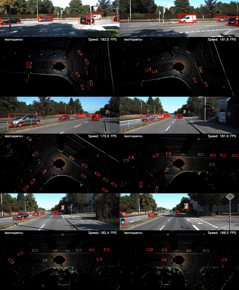
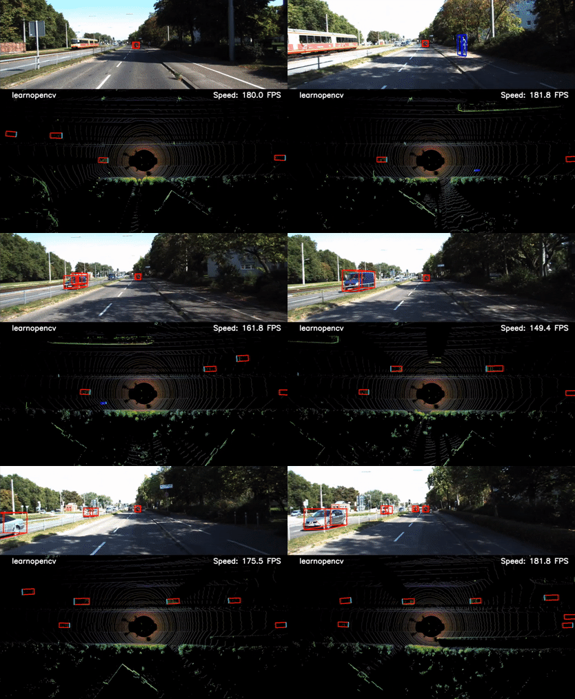
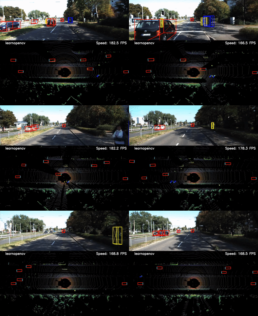
In this section of the research article, we will explore the inference results from this experiment:
Analysis of Experimental Results
Based on the inference visualizations obtained from the experiments, the following observations can be made:
- BEV Map: The localized objects are detected from a top-down BEV 3D LiDAR depth map, generated by the sensor. This has both the front and back views concatenated as one whole map.
- Three-class 3D Object Detection: Predefined classes such as cars, pedestrians and cyclists are detected in the inference result. These classes were pre-annotated in the KITTI 360 Vision dataset.
- Localization Accuracy: 3D bounding boxes are used to visualize the detected objects, in both the modalities i.e. 2D RGB camera and 3D LiDAR sensor. Not just that, but it can also be observed that the accuracy in the bounding box placement in both the streams are accurate.
- Real-time Performance: The inference pipeline was tested on the same deep learning machine in which this model was trained on, which is powered by an NVIDIA RTX 3080 Ti with 12GB vRAM. In this case, the model achieved a consistent 160-180 FPS performance during real-time inference, as shown in FIGURE 13 to FIGURE 15.
Analysis of Evaluation Metrics
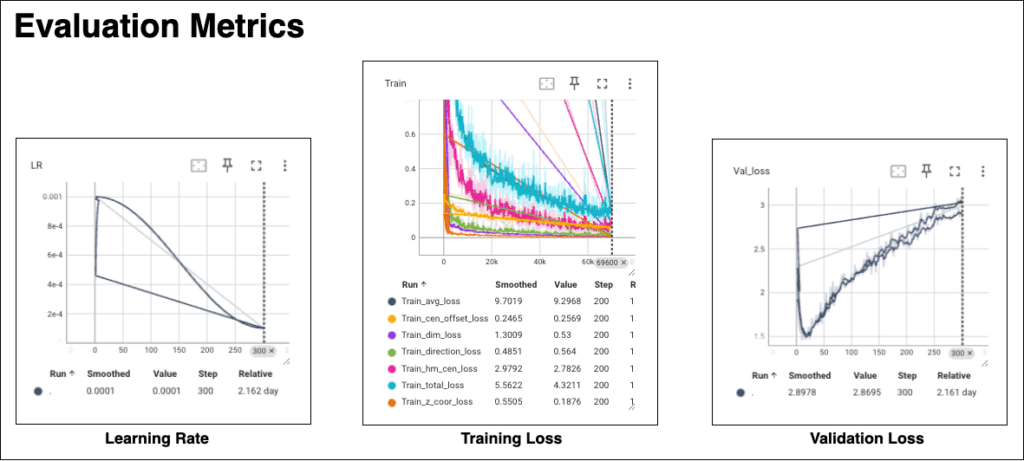
In the previous sections, we were able to get an understanding of the visual results of the trained model. But there are many opportunities to improve this model’s performance, as well. For this, let’s look at the evaluation metrics, which were logged during the training process using TensorBoard.
Learning Rate
The learning rate (LR) graph depicts a step decay schedule, beginning just below 0.001 and progressively declining to approximately 0.0001 by step 300. Sharp reductions at specific intervals suggest predetermined epochs for significant LR decreases. Between these drops, the LR plateaus, allowing the model to stabilize its learning. The graph indicates a balance between initial rapid learning and subsequent fine-tuning, following common LR scheduling practices in model training.
Training Loss
In this specific experiment, the K-FPN model was trained for a total of 300 epochs, and the training loss graph depicts multiple decreasing trends, with initial high losses indicating early learning stages. As training progresses, all loss metrics, including avg_loss, cen_offset_loss, and total_loss, consistently decline, signaling model improvement. Notably, the loss curves begin to plateau around 69k steps, suggesting the model is nearing convergence. The composite total_loss also demonstrates a downward trajectory, reflecting the cumulative benefit of individual loss optimizations.
Validation Loss
On the other hand, the validation loss graph exhibits an initial decline followed by a consistent rise, hinting at early learning success but subsequent overfitting. Persistent upward trends post 50 steps suggest diminishing model generalizability. Fluctuations in the loss indicate variability in learning, with the final validation loss settling around 2.8695, higher than its minimum, confirming reduced performance on unseen data over time.
To enhance your understanding and engage hands-on with the code, take a walk through the code here.
Conclusions
This experimental investigation into 3D LiDAR object detection using the Keypoint Feature Pyramid Network (K-FPN) model has yielded several key insights. The model demonstrates robust object localization capabilities within BEV maps, integrating front and back views from 3D LiDAR depth maps for comprehensive coverage. The accuracy of object detection is noteworthy, with the system effectively identifying and placing bounding boxes around cars, pedestrians, and cyclists—three critical classes within the KITTI 360 Vision dataset.
In terms of performance, the model’s real-time inference, tested on an NVIDIA RTX 3080 Ti, shows impressive results, consistently achieving 160-180 FPS, underscoring the model’s potential for deployment in real-world applications where rapid processing is crucial. The training loss trends observed during the 300 epochs underscore a successful learning phase, with all loss metrics indicating steady improvement and approaching convergence. This contrasts with the validation loss, which, after an initial dip, shows an increase, signaling potential overfitting beyond the 50-step mark. The divergence between training and validation loss suggests that while the model learns the training data effectively, its generalization to new data needs further enhancement.
The research conducted and the results obtained have significant implications for the advancement of ADAS and autonomous navigation systems. The model’s efficacy in accurate and fast object detection opens pathways for improved safety and efficiency in autonomous vehicle technology. Moving forward, addressing the challenges of overfitting and ensuring the model’s generalization remains a priority, with the potential for exploring more sophisticated regularization techniques or adaptive learning rate schedules to optimize model performance on unseen datasets.
References
[1] S. Ji, W. Xu, M. Yang and K. Yu, “3D Convolutional Neural Networks for Human Action Recognition,” in IEEE Transactions on Pattern Analysis and Machine Intelligence, vol. 35, no. 1, pp. 221-231, Jan. 2013, doi: 10.1109/TPAMI.2012.59.
[2] Zhou, Yin, and Oncel Tuzel. “Voxelnet: End-to-end learning for point cloud based 3d object detection.” Proceedings of the IEEE conference on computer vision and pattern recognition. 2018.
[3] Beltrán, Jorge, et al. “Birdnet: a 3d object detection framework from lidar information.” 2018 21st International Conference on Intelligent Transportation Systems (ITSC). IEEE, 2018.
[4] Wu, Hai, et al. “Virtual Sparse Convolution for Multimodal 3D Object Detection.” Proceedings of the IEEE/CVF Conference on Computer Vision and Pattern Recognition. 2023.
[5] Li, Peixuan, et al. “Rtm3d: Real-time monocular 3d detection from object keypoints for autonomous driving.” European Conference on Computer Vision. Cham: Springer International Publishing, 2020.
[6] Nguyen, M. D. (2020). Super-Fast-Accurate-3D-Object-Detection-PyTorch.
[7] Geiger, A., Lenz, P., & Urtasun, R. (2012). Are we ready for Autonomous Driving? The KITTI Vision Benchmark Suite. In Conference on Computer Vision and Pattern Recognition (CVPR).

