YOLOv6 Custom Dataset Training – Underwater Trash Detection

The field of object detection is coming across a new YOLO model release every few months. Although reading the paper should be the first step towards exploring the model, we can evaluate the model properly only after training it on a custom dataset. YOLOv6 recently released version 2.0 of all its models. In this article, we will be performing a YOLOv6 custom dataset training.

As per the publication, YOLOv6 is meant for industrial object detection applications. This implies that all the YOLOv6 models should perform well even on datasets that are not similar to the COCO dataset.

The repository also provides models which have been trained for longer (400 epochs). Further, the codebase has ONNX version of the models. All these will help towards easier adaptation of YOLOv6 for industrial applications. For this reason, we choose a fairly difficult dataset for solving a real-life problem: An underwater trash detection dataset that aims to facilitate trash detection on deep ocean floors.

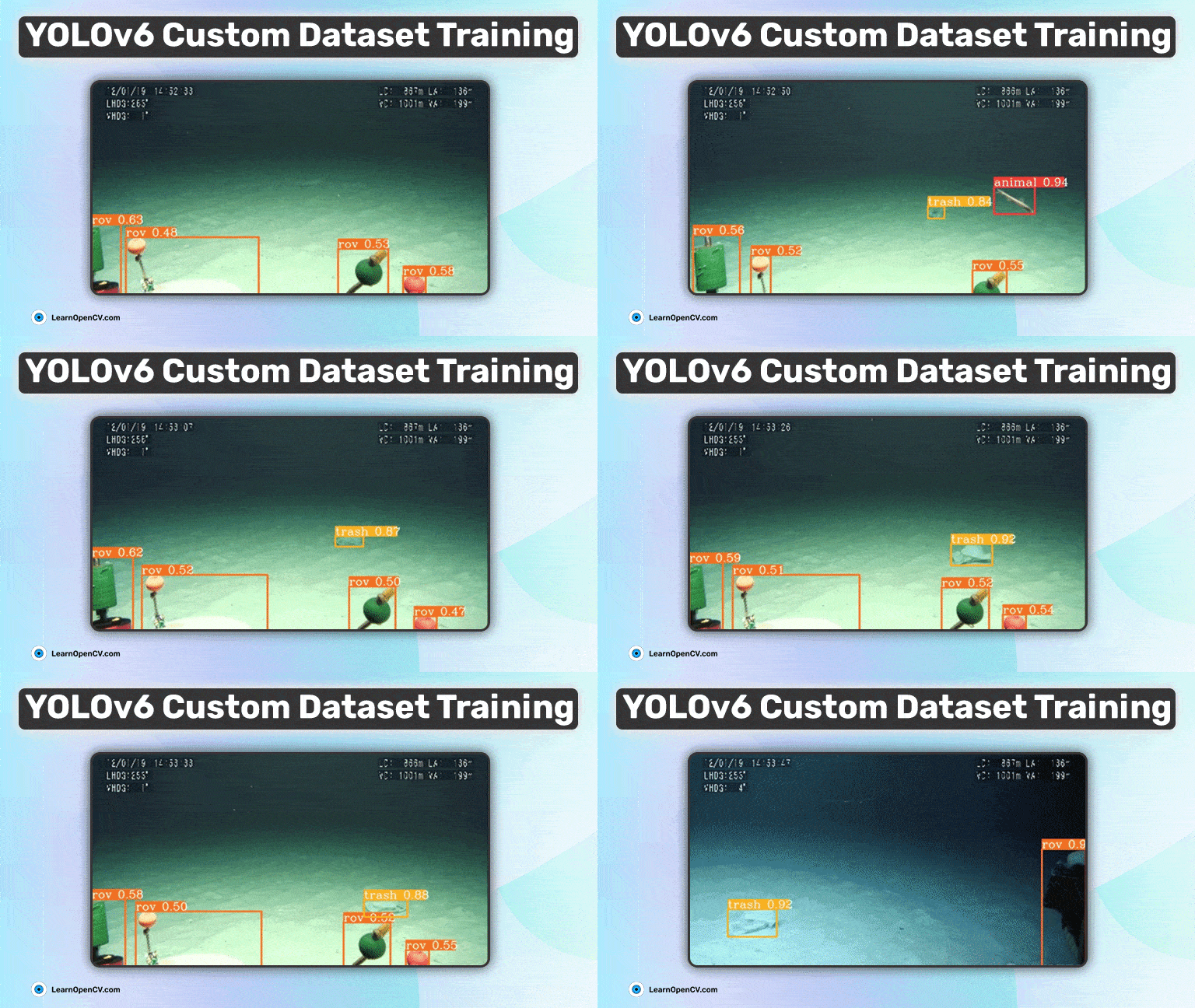
The following GIF shows the detection outputs from the validation dataset after training the YOLOv6 Large model.

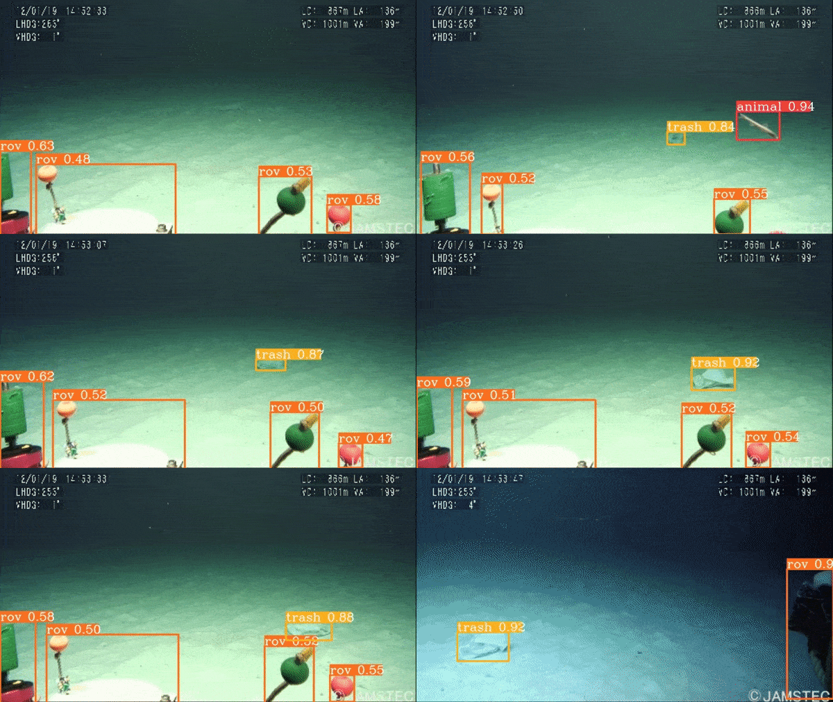
To know the details of the dataset and the procedure for training YOLOv6 on a custom dataset, follow along.

But before that, if you are keen to learn more about YOLOv6,  we encourage you not to miss the YOLOV6 object detection paper explanation article. It will give you in-depth insight into the architecture, different YOLOv6 models, and the performance on the COCO benchmark dataset.

• What are the Models Available in YOLOv6?
• The TrashCan Dataset
• YOLOv6 Custom Dataset Training
• YOLOv6 vs YOLOv5 vs YOLOv7
• Conclusion

YOLO Master Post –  Every Model Explained

Unlock the full story behind all the YOLO models’ evolutionary journey: Dive into our extensive pillar post, where we unravel the evolution from YOLOv1 to YOLO-NAS. This essential guide is packed with insights, comparisons, and a deeper understanding that you won’t find anywhere else.
Don’t miss out on this comprehensive resource, Mastering All Yolo Models for a richer, more informed perspective on the YOLO series.

Mastering All YOLO Models from YOLOv1 to YOLO-NAS: Papers Explained (2024)

What are the Models Available in YOLOv6?

As of writing this, YOLOv6 contains 5 major models. Each of them targets a particular set of computation devices (edge GPU, desktop GPU, or cloud GPU) according to their specified number of parameters.

All the YOLOv6 models have been pre-trained on the COCO object detection dataset. You can find the pre-trained weights on the official GitHub repository.

There is also a YOLOv6 Large model trained with the ReLU activation [1], which tends to be faster but with a slightly lower mAP (51.7).

Other than these, you can also find a list of quantized models in the official repository.

To solve the underwater trash detection problem, we will use three models, which are:

• YOLOv6n (YOLOv6 Nano)
• YOLOv6s (YOLOv6 Small)
• YOLOv6l (YOLOv6 Large)

Training the above three models on the dataset and analyzing the results will give us a proper idea of which model to use. Also, it will help us uncover the advantages and disadvantages of using large models when it is not absolutely necessary.

The TrashCan Dataset

The TrashCan (1.0) dataset is composed of images annotated for detecting trash, ROVs, and flora & fauna on the ocean floors.

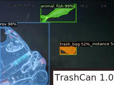
This dataset is part of a research that also has an accompanying technical article. It contains 7212 images with annotations, for instance, segmentation and bounding box detection. 

Training deep learning models on such a dataset can help recognize and localize trash in deeper parts of the ocean in an easy manner.

The TrashCan dataset contains two versions. They are:

• TrashCan-Material: Contains 16 different classes.
• TrashCan-Instance: Contains 22 different classes.

You can find the names of all the classes in the TrashCan 1.0 research article. In this tutorial, we use a modified version of the TrashCan Material Version of the dataset. Instead of using all 16 classes, we boil it down to only 4. They are: 

• Animal (all animals like eel, fish, crab, etc.)
• Plant
• ROV
• Trash (All trash objects like fabric, metal, plastic, etc.)

The above modification to the dataset serves two purposes. On the one hand, it reduces the dataset complexity, and on the other, it keeps the visualization space quite simple. It can be difficult to keep visual track of objects which look very similar (e,g. different categories of trash). Hence reducing them to just 4 classes helps in easier visualization.

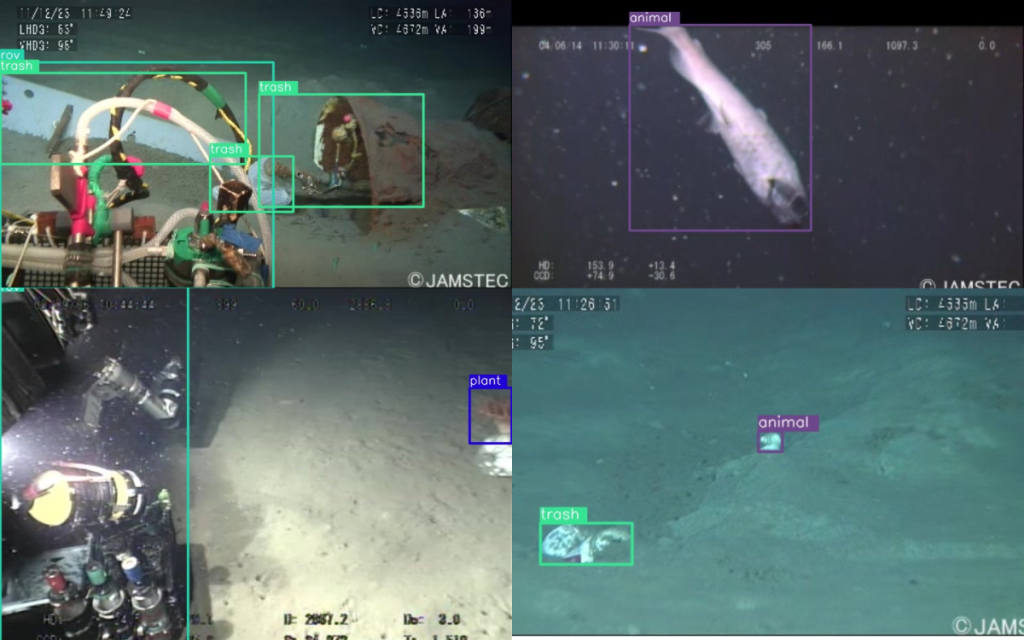
The above figure shows images with the modified classes.

YOLOv6 Custom Dataset Training

Let’s jump into the practical side of the tutorial without any further delay. Training YOLOv6 on a custom dataset (underwater trash detection dataset) involves the following steps:

• Download and prepare the underwater trash detection dataset.
• Clone the YOLOv6 repository.
• Create the YAML file for the dataset. This includes the paths to the training and validation images, as well as the class names.
• Download the YOLOv6 COCO pretrained weights.
• Execute the training command with the required arguments to start the training. For fine tuning YOLOv6 on a custom dataset, it can be as simple as the following.
  • python tools/train.py --epochs 100 --batch-size 32 --conf configs/yolov6n_finetune.py --data data/data.yaml

Let’s begin by downloading the dataset.

Download the Underwater Trash Detection Dataset

The dataset that we will use here has only four classes. It has already been modified.

If you are on Linux, you can execute the following commands in the terminal to download and extract the dataset.

wget https://www.dropbox.com/s/lbji5ho8b1m3op1/reduced_label_yolov6.zip?dl=1

unzip reduced_label_yolov6.zip

This article also has an accompanying Jupyter notebook. You can upload it on either Kaggle or Colab to execute them, irrespective of the operating system that you are using.

Clone the YOLOv6 Repository

The next step is to clone the YOLOv6 repository and install the requirements.

https://github.com/meituan/YOLOv6.git

pip install -r requirements.txt

Creating the Underwater Trash Detection Dataset YAML File

Just like any other YOLO training procedure, we need a dataset YAML file for YOLOv6 as well. This contains the paths to the training and validation images, the number of classes, and the class names.

Click here to download the source code to this post

# Please insure that your custom_dataset are put in same parent dir with YOLOv6_DIR
train: 'reduced_label_yolov6/images/train' # train images
val: 'reduced_label_yolov6/images/valid' # val images

# whether it is coco dataset, only coco dataset should be set to True.
is_coco: False
# Classes
nc: 4  # number of classes
names: [
    'animal',
    'plant',
    'rov',
    'trash'
]  # class names

The training and validation images are inside their respective directories. Exploring the dataset directory will reveal the following structure:

├── images
│   ├── train
│   └── valid
└── labels
    ├── train
    └── valid

The label text files are present inside the labels directory. You may also notice an is_coco attribute in the YAML file. In YOLOv6, this informs the training script whether the dataset is a COCO dataset or not. This attribute can take a boolean value.

Download the YOLOv6 Pretrained Weights

Before we start the training, we need to download the weights that have already been pretrained on the COCO dataset. Generally, pretrained models lead to faster convergence.

The following code block shows how to create a weights directory inside the cloned repository and download the weights.

YOLOv6n pretrained weights

wget https://github.com/meituan/YOLOv6/releases/download/0.2.0/yolov6n.pt -O weights/yolov6n.pt

YOLOv6s pretrained weights

wget https://github.com/meituan/YOLOv6/releases/download/0.2.0/yolov6s.pt -O weights/yolov6s.pt

YOLOv6m pretrained weights

wget https://github.com/meituan/YOLOv6/releases/download/0.2.0/yolov6l.pt -O weights/yolov6l.pt

As we will be training the YOLOv6 Nano, Small, and Large models, we will be downloading all the pretrained weights here.

Training YOLOv6 Nano on Custom Dataset

All the training and inference experiments that we show here were done on a cloud GPU with the following hardware:

• AMD EPYC 7542 processor
• 32 GB RAM
• 2x Tesla V100 (16GB) GPU – total 32 GB VRAM

The results shown in this post are from distributed training (2x V100 GPU). However, one can easily start training on a single GPU as well.

The article contains both commands to train on two GPUs as well to train on a single GPU.

To start the training of YOLOv6n in a distributed manner (PyTorch Data Parallel), one can execute the following command:

python tools/train.py \
--epochs 100 \
--batch-size 32 \
--conf configs/yolov6n_finetune.py \
--data data/underwater_reduced_label.yaml \
--write_trainbatch_tb \
--device 0,1 \
--eval-interval 1 \
--img-size 640 \
--name v6n_32b_640img_100e_reducedlabel

Let’s go over the important command line arguments:

• --epochs: Number of epochs to train for.
• --batch-size: Number of training samples in one batch of data.
• --conf: The model configuration to use. We are using the yolov6n_finetune.py here, which already comes with the YOLOv6 repository, for fine-tuning purposes.
• --data: The dataset YAML file.
• --write_trainbatch_tb: It is a boolean argument indicating that we want to write the logs to TensorBoard.
• --device: This takes the GPU device IDs. As we are running multi-GPU training, the value is 0,1 (no space after the comma).
• --eval-interval: Number of epochs after which to run the pycocotools evaluation. We are running the evaluation after each epoch.
• --img-size: Image size for training.
• --name: The project directory name. Giving a suitable name will help to easily distinguish between the training experiments.

If you want to run the training on a single GPU, you can assign a value of either 0 or 1 or 2, or 3, depending on the GPU you want to run the training on. 

The following command is an example of running the training on GPU device 0.

python tools/train.py \
--epochs 100 \
--batch-size 32 \
--conf configs/yolov6n_finetune.py \
--data data/underwater_reduced_label.yaml \
--write_trainbatch_tb \
--device 0 \
--eval-interval 1 \
--img-size 640 \
--name v6n_32b_640img_100e_reducedlabel

The training will take a few hours to run and will vary depending on the hardware that you run it on.

YOLOv6 Nano Training Results and Inference

The following is the mAP plot at o.50:00.95 IoU from the validation loop of the training process.

The highest mAP that we got was 0.488 (48.8).

We can also run the validation using the evaluation script with the following command.

python tools/eval.py \
--data data/underwater_reduced_label.yaml \
--weights runs/train/v6n_32b_640img_100e_reducedlabel/weights/best_ckpt.pt \
--name yolov6n_eval \
--verbose

Notice that we are using the best checkpoint here. Also, the --verbose command ensures that the class-wise average precision is also shown. The following is the output from the terminal.

Class           Labeled_images      Labels     [email protected]     [email protected]    [email protected]      [email protected]  [email protected]:.95
all                     1149        2420       0.765        0.63       0.691       0.724       0.488
animal                   304         523        0.66        0.53       0.588       0.574       0.317
plant                     98         102       0.684        0.63       0.656       0.582       0.318
rov                      436         589        0.94        0.82       0.876       0.922       0.758
trash                    940        1206       0.894        0.73       0.804       0.817        0.56

To take it ahead, let’s run inference on a few videos. After training the model, you may run inference on your own videos as well by changing the file path in the following command.

python tools/infer.py \
--weights runs/train/v6n_32b_640img_100e_reducedlabel/weights/best_ckpt.pt  \
--yaml data/underwater_reduced_label.yaml \
--source data/underwater_inference_data/manythings.mp4 \
--name v6n_video_infer \
--view-img

When running inference on a YOLOv6 model trained on custom datasets, we need to take care of the following commands:

• --weights: The path to the correct weights.
• --yaml: This accepts the path to the custom dataset YAML file.
• --source: Path to the images/videos/or directory containing inference data.
• --view-img: This is a boolean flag indicating that we want to visualize the results on the screen.

All the inference experiments were run on a laptop GTX 1060 GPU with 6GB of VRAM.

The following are output results from YOLOv6 Nano inference.

In the first video, the Nano model is missing out on detecting the ROV in all frames. It is also unable to detect the crab  (belonging to animal class) in the final frames. In the second video, although it can detect the trash correctly, the detections for the fish fluctuate.

This is a challenging dataset, and a Nano model may not be enough. One upside is that we are getting more than 140 FPS here. Next, we will train YOLOv6 Small and Large models and check the performance.

Training YOLOv6 Small Model on Custom Dataset

Training the YOLOv6s model requires very minimal changes to the training command.

python tools/train.py \
--epochs 100 \
--batch-size 32 \
--conf configs/yolov6s_finetune.py \
--data data/underwater_reduced_label.yaml \
--write_trainbatch_tb \
--device 0 \
--eval-interval 1 \
--img-size 640 \
--name v6s_32b_640img_100e_reducedlabel

YOLOv6 Small Training Results and Inference

The following is the mAP graph from TensorBoard.

We can see that the mAP was increasing till the end of the training. A longer training will perhaps help achieve better mAP.

The following are the class-wise AP after running the evaluation script.

Class           Labeled_images      Labels     [email protected]     [email protected]    [email protected]      [email protected]  [email protected]:.95
all                     1149        2420       0.798        0.65       0.716       0.764       0.526
animal                   304         523       0.717        0.61       0.659       0.654       0.374
plant                     98         102       0.805         0.6       0.688       0.634       0.369
rov                      436         589       0.962        0.85       0.902       0.947       0.791
trash                    940        1206       0.876        0.75       0.808       0.821       0.571

As expected, we have a higher mAP of 0.526 when training with the smaller model compared to the nano model.

Let’s examine the inference results to see how the YOLOv6 Small model performs on unseen data.

This time the trash detection results look more stable with fewer fluctuations and higher confidence. Still, the crab detection at the end of the video (top one) is not that good. Maybe training the YOLOv6 large model will help.

YOLOv6 Large Custom Dataset Training

Similar to the previous two training experiments, we only need to change the fine-tuning module path to carry out the YOLOv5 large training.

python tools/train.py \
--epochs 100 \
--batch-size 32 \
--conf configs/yolov6l_finetune.py \
--data data/underwater_reduced_label.yaml \
--write_trainbatch_tb \
--device 0 \
--eval-interval 1 \
--img-size 640 \
--name v6l_32b_640img_100e_reducedlabel

The large model utilizes much more GPU memory compared to the previous two models. In case you run into OOM (Out Of Memory) error, consider reducing the batch size to 16 or 8.

YOLOv6 Large Training Results and Inference

The following is the mAP plot for the YOLOv6 large model training from TensorBoard.

It is clear that the large model’s mAP plateaus by the end of the training. But that’s not all. Looking at the following mAP values reveals something more.

Class           Labeled_images      Labels     [email protected]     [email protected]    [email protected]      [email protected]  [email protected]:.95
all                     1149        2420       0.813        0.66       0.728       0.776       0.555
animal                   304         523       0.713        0.66       0.686       0.689       0.401
plant                     98         102        0.79        0.62       0.695       0.636       0.413
rov                      436         589       0.896        0.92       0.908       0.944       0.813
trash                    940        1206       0.874        0.78       0.824       0.837       0.592

Out of three YOLOv6 models, YOLOv6 Large gives the highest mAP of 0.555. Hopefully, we can get similar results during inference as well.

The YOLOv6 Large model is producing excellent results in the two videos. This is evident because It can detect the crab pretty well at the end of the first video. And the detection of the two fish in the second video is much more consistent.

YOLOv6 vs YOLOv5 vs YOLOv7

For comparison purposes, we also trained the YOLOv5 Extra Large model and the YOLOv7 model on the same dataset. We will compare it with the results of the YOLOv6 Large model as they have the most comparable mAPs when pretrained on the COCO dataset.

The hyperparameters while training the YOLOv5 and YOLOv6 models were kept very much similar to the YOLOv6 training as possible. They were trained for 100 epochs with a batch size of 32 on two GPUs with Data Parallel.

The following video has been taken from YouTube to show a fair comparison between the three models.

Undoubtedly, the YOLOv6 Large model seems to perform the best here. Apparently, the updated YOLOv6 models and methods are holding up to expectations.

Conclusion

In this article, we carried out YOLOv6 training on a custom dataset. We chose the underwater trash detection dataset for this purpose.

• We began by understanding the dataset and preparing the dataset YAML file.
• Then we moved on to preparing the YOLOv6 codebase for the custom training purpose.
• After downloading the pretrained weights, we trained the YOLOv6n, YOLOv6s, and YOLOv6l models.
• We also ran inferences on unseen videos to evaluate their qualitative results.
• Finally, we compared the YOLOv6 Large model with the YOLOv5 Extra Large and YOLOv7 models.

If you extend the project in any manner, let us know in the comment section how it performed and what insights you gained from it. We would love to hear from you!

Must Read Articles

References

[1] Deep Learning using Rectified Linear Units (ReLU)