YOLO11 on Raspberry Pi: Optimizing Object Detection for Edge Devices

Imagine you have multiple warehouses in different places where you don’t have time to monitor everything at a time, and you can’t afford a lot of computes due to their cost and unreliability. However, using cloud-based systems is also not ideal; they can be slow or stop working sometimes and can be expensive, too. That’s where edge computing helps. Instead of sending data back and forth to faraway servers, edge computing lets you process everything locally, right where it happens. One of the best low-cost solutions for this setup is using a YOLO11 on Raspberry Pi.

In this article, we’ll explore how YOLO11 on Raspberry Pi revolutionizes computer vision and object detection for resource-constrained environments. We’ll see how you can achieve real-time performance, minimal latency, and high accuracy, all on a device that sits in the palm of your hand.

In this article, we will explore:

• Why edge devices like the Raspberry Pi are crucial for modern AI deployments
• How YOLO11 builds upon previous YOLO versions to offer higher speed and optimized performance
• Key hardware and software strategies for bringing YOLO11 to life on the Raspberry Pi
• Practical benefits of running object detection locally, from bandwidth savings to near-instant response times.
• Common challenges and solutions when implementing object detection on the edge

Now, that’s exciting, right? So, grab a cup of coffee, and let’s dive in!

TL;DR – Blog Highlights

Edge AI on the Rise: The global Edge AI market will reach USD 206 billion by 2032, growing at an 18.3% CAGR, underscoring the importance of on-device processing for real-time applications.

Why Raspberry Pi? With its compact size, low power consumption, and improved CPU/VideoCore VII GPU, specs (especially on the Raspberry Pi 5), this credit-card-sized computer is perfect for deploying AI at the network edge.

YOLO11 Advantages: As the latest iteration of the You Only Look Once series, YOLO11 offers a significantly reduced model complexity (up to 37% less than YOLOv8) while retaining 54.7% mAP, enabling real-time object detection on resource-constrained hardware.

Speed & Efficiency: When optimized for Raspberry Pi using techniques like NCNN model conversion and hardware-aware quantization, YOLO11 can achieve millisecond-level latency and handle up to 25+ FPS on 240×240 resolution frames.

Don’t worry if all this sounds technical; we’ve got you covered. You can grab our complete Python scripts and implementation details to get started swiftly. Hit the “Download Code” button (coming soon in the blog) for an effortless dive into YOLO11 on Raspberry Pi.

Introduction to Raspberry Pi

The Raspberry Pi started out as a credit-card-sized computer aimed at sparking interest in basic computer science, but it has since evolved into a go-to platform for all sorts of applications, including edge AI. Released in 2012 by the Raspberry Pi Foundation, the original model cost just $35 and immediately became a sensation among hobbyists, educators, and professionals. Fast-forward to today, and the Raspberry Pi lineup has sold over 60 million units, each iteration more powerful than the last.

A Quick Overview of Raspberry Pi Generations

• Raspberry Pi 1: The pioneer of low-cost, single-board computing, with modest processing power suitable for light tasks and educational projects.
  
• Raspberry Pi 2 and 3: Substantial CPU upgrades, increased RAM, and built-in Wi-Fi/Bluetooth connectivity paved the way for lightweight server tasks, robotics, and early AI experiments.
  
• Raspberry Pi 4: Introduced USB 3.0 ports, up to 8GB RAM, and a more powerful GPU, broadening the scope for computer vision, media centers, and more sophisticated applications.
  
• Raspberry Pi 5: The latest model has a 2.4 GHz quad-core ARM Cortex-A76 processor, refined VideoCore VII GPU, support for PCIe connectivity, and LPDDR4X-4267 SDRAM in 4GB or 8GB configurations.

Why Raspberry Pi Is Ideal for Edge AI

1. Cost-Effectiveness: Priced under $100 (often around $50 for the base Pi 5), it’s feasible to deploy multiple units across various locations. Imagine outfitting an entire factory floor with these tiny boards for distributed real-time analytics—without breaking the bank.
   
2. Robust Community & Support: Open-source documentation, countless forums, and community-driven libraries make troubleshooting easier. For example, tools like picamera2 or libcamera provide direct integration for camera modules, letting you capture image data for YOLO-based inference almost instantly.
   
3. Improved Hardware Acceleration: With each new iteration, Raspberry Pi gains better hardware acceleration capabilities. The Pi 5’s enhanced GPU, coupled with potential additions like Google Coral USB accelerators, can provide the extra boost needed for more demanding YOLO11 variants.

P.S. We are using the Raspberry Pi 5(8 GB) for this article.

Our courses cover Object Detection, Fundamentals of Computer Vision, and Deep Learning in depth. To get started, just click below on any of our free Bootcamps!

Why We Are Using YOLO11

If you’ve followed the YOLO (You Only Look Once) family of models, you know they’ve made a name by combining high accuracy with real-time object detection. Each new iteration—YOLOv3, YOLOv5, YOLOv8, and so forth has introduced better architecture to tackle computer vision tasks faster and more efficiently. Now, YOLO11 pushes these optimizations even further, and here’s why it stands out for edge computing on a device like the Raspberry Pi:

Low Latency: Thanks to architectural enhancements like the C3k2 and C2PSA blocks, YOLO11 doesn’t just detect objects accurately; it does so at millisecond-level latency. That’s vital in scenarios where quick decisions save time, resources, or even lives (think drones, robotics, or security systems).

NCNN Integration: By converting PyTorch weights to the NCNN format (designed specifically for edge devices), you can slash inference times by up to 62%, making real-time detection more than just a theoretical possibility.

Maintained mAP: Even though YOLO11 is lighter, it still maintains around 55% mAP on common object detection benchmarks. This balance between speed and accuracy ensures you’re not sacrificing detection quality for efficiency.

We’re using YOLO11 on the Raspberry Pi because it hits the sweet spot of speed, accuracy, and resource efficiency. Traditional solutions might have required hefty GPUs or large compute clusters to achieve real-time results, but YOLO11 runs right at the edge—no extra hardware accelerators necessary (though you can add them if you like).

Download the Code Here

Click here to download the source code to this post

Code Pipeline

Now, let’s jump into the code. First, we will start with creating the environment:

! conda create -n yolo11xrpi python=3.11
! conda activate yolo11xrpi
! pip install ultralytics

After the environment is set up, we will export the Yolo11 model to get the best FPS in Raspberry Pi. Ultralytics provides several export options; we will focus on: OpenVINO, NCNN, and MNN. We will use YOLO11n and YOLO11s variants. 

OpenVINO (Open Visual Inference and Neural Network Optimization) is Intel’s toolkit for optimizing and deploying neural networks, especially on Intel hardware. While OpenVINO is primarily tailored for CPUs, VPUs, and GPUs from Intel, it also offers support for ARM devices, including Raspberry Pi. 

NCNN is a high-performance neural network inference framework developed by Tencent, specifically designed for mobile and edge devices using ARM architecture. It is extremely lightweight and requires minimal dependencies, making it a great choice for direct deployment on Raspberry Pi. 

MNN (Mobile Neural Network), developed by Alibaba, is another robust inference framework optimized for mobile and embedded platforms. Like NCNN, MNN is lightweight and supports a variety of optimizations, including quantization and GPU acceleration through OpenCL or Vulkan. 

We will use this command to export YOLO11 models into our required format:

yolo export model=yolo11n.pt format=ncnn #export in any format 

We are using the ultralytics export command. For all the available parameters, visit the ultalytics docs.

We will use the YOLO11n for the blog as our main focus is to use less storage and deliver more accuracy and FPS. Now, let’s move the main code:

Imports and Setup

import cv2
import numpy as np
import time
from ultralytics import YOLO

from collections import defaultdict

We start by importing the essential libraries:

• OpenCV (cv2) for handling video frames, drawing bounding boxes, and showing results in windows.
  
• NumPy (np) for numerical operations and array handling.
  
• time to measure the duration of each loop (for computing FPS).
  
• YOLO from the ultralytics package, our key deep learning model for detection and tracking.
  
• defaultdict from Python’s collections, which helps us store tracking data without manually checking if keys exist.
  

Defining the inference Function

def inference(
    model,
    mode,
    task,
    video_path=None,
    save_output=False,
    output_path="output.mp4",
    show_output=True,
    count=False,
    show_tracks=False,
):

The inference(...) takes a model (YOLO instance), the mode (webcam or video file), the task (detect or track), and several optional parameters for saving the output, showing the result on screen, and whether to count or draw the trajectories of objects.

Pre processing

    if mode == "cam":
        cap = cv2.VideoCapture(0)
    elif mode == "video":
        if video_path is None:
            raise ValueError("Please provide a valid video path for video mode.")
        cap = cv2.VideoCapture(video_path)
    else:
        raise ValueError("Invalid mode. Use 'cam' or 'video'.")

    # History for tracking lines
    track_history = defaultdict(lambda: [])

    # History for unique object IDs per class (used in tracking count)
    seen_ids_per_class = defaultdict(set)

    fourcc = cv2.VideoWriter_fourcc(*"mp4v")
    input_fps = cap.get(cv2.CAP_PROP_FPS)
    out = None

First, we create the VideoCapture object. Then, we create two defaultdict objects:

• track_history to remember all the (x, y) coordinates for each tracked object ID. This lets us draw a path of where the object has been.
  
• seen_ids_per_class to keep a set of object IDs for each class (like “person,” “car,” etc.), helping us count unique objects.

We create a VideoWriter object to save the processed video frames later on.

Main Processing Loop

    while cap.isOpened():
        success, frame = cap.read()
        if not success:
            print("Failed to read frame or end of video")
            break

        start_time = time.time()
        class_counts = defaultdict(int)

        # Inference
        if task == "track":
            results = model.track(frame, conf=0.3, persist=True, tracker="bytetrack.yaml")
        elif task == "detect":
            results = model.predict(frame, conf=0.5)
        else:
            raise ValueError("Invalid task. Use 'detect' or 'track'.")

        end_time = time.time()
        annotated_frame = results[0].plot()

In this section of code, we’re inside a loop that runs as long as our capture device (webcam or video file) is open. We begin by reading a frame (success, frame = cap.read()), and if there’s no more data to read, we break out with a message indicating the end of the feed. Next, we note down the start time (start_time = time.time()), which allows us to measure how long it takes to process this frame. It is useful for calculating frames per second later. We then prepare a dictionary (class_counts) to track how many times each object class appears, though we only actually use it if we’re in detection mode and counting is enabled. 

Depending on whether we’re doing tracking or detection, we call model.track or model.predict. In tracking mode, we specify a confidence threshold (conf=0.3), keep object identities persistent across frames (persist=True), and use a specific tracking configuration file (“bytetrack.yaml“). In detection mode, we perform a straightforward prediction with a slightly higher confidence threshold (conf=0.5). We mark the end time (end_time = time.time()) to compute how long inference took, and finally, we create an annotated version of the frame (annotated_frame = results[0].plot()) with bounding boxes and labels overlaid, ready for display or saving.

YOLO’s Output Tensors

When we run either model.track() or model.predict(), YOLO returns a list called results. Since our code processes one image (or one frame) at a time, we typically focus on results[0], which holds the detections for that single frame.

Within results[0], you’ll often see something like:

results[0].boxes

This boxes object contains several useful pieces of information about each detection:

1. Coordinates:
   
   • boxes.xywh gives bounding box coordinates in the format (x_center, y_center, width, height).
     
   • These coordinates can be on the CPU or GPU, so we often convert them to CPU with .cpu() if we want to handle them in NumPy or standard Python.
     
2. Class Indices (boxes.cls):
   
   • YOLO assigns each detection a class index (e.g., 0 for “person,” 1 for “bicycle,” etc.).
     
   • In our code, we do something like class_ids = results[0].boxes.cls.int().cpu().tolist() to convert this tensor into a regular Python list of integers.
     
   • We then map these integer IDs to actual class names using names = results[0].names.
     
3. Tracking IDs (boxes.id):
   
   • Only available when we use model.track().
     
   • Each detected object across consecutive frames gets a unique integer ID so we can tell it’s the same object in the next frame.
     
   • We do track_ids = results[0].boxes.id.int().cpu().tolist() to store those IDs as a Python list for easy looping.
     

These three things, coordinates, class indices, and (optionally) track IDs are the main items we need to handle detection, counting, and tracking.

Detection and Class Indexing

if task == "detect":
    results = model.predict(frame, conf=0.5)

...
if results[0].boxes and results[0].boxes.cls is not None:
    boxes = results[0].boxes.xywh.cpu()
    class_ids = results[0].boxes.cls.int().cpu().tolist()
    names = results[0].names

1. model.predict(frame, conf=0.5) returns a tensor of detections.
   
2. results[0].boxes.cls is where we get the class indices for each bounding box. We convert those class indices into integers and move them to the CPU for easy handling.
   
3. names = results[0].names is a list or dictionary inside the YOLO model that maps each integer ID to a readable class name (like “person,” “cat,” or “car”).
   

When we’re only detecting (no tracking), each frame is independent. If we also want to count how many objects of each class appear in a single frame, we can do something like:

class_counts = defaultdict(int)

for cls_id in class_ids:
    class_counts[names[cls_id]] += 1

Here, we loop through the class_ids and simply increment a count in class_counts for the corresponding class name. This is how the code knows, for example, that in a particular frame, we have 3 cars, 2 people, and 1 traffic light.

Tracking with Unique IDs

if task == "track":
    results = model.track(frame, conf=0.3, persist=True, tracker="bytetrack.yaml")

...
if task == "track" and results[0].boxes.id is not None:
    track_ids = results[0].boxes.id.int().cpu().tolist()
    
    for box, cls_id, track_id in zip(boxes, class_ids, track_ids):
        x, y, w, h = box
        class_name = names[cls_id]
        ...

When we switch to tracking mode (task == "track"), YOLO automatically adds a tracking ID (.id) for each detection. This is the key difference from simple detection:

1. boxes.id holds a tensor of IDs, one for each bounding box in the current frame. We just convert them into a list and store them as track_ids.

2. We loop over zip(boxes, class_ids, track_ids) to simultaneously process:
   
   • The bounding box coordinates (x, y, w, h)
     
   • The class ID (cls_id)
     
   • The tracking ID (track_id)
     

At this point, we can decide to store these tracking IDs somewhere to keep track of them across frames. In the provided code, we’re updating:

• seen_ids_per_class[class_name].add(track_id) if we want to count unique objects of each class. That way, the same car or person keeps the same ID and isn’t double-counted.
  
• track_history[track_id] if we want to draw a path (trajectory) for each tracked object. We append (x, y) each time we see the same track_id, then draw lines connecting those points.
  

This is how the code knows the same “car #5” is present across multiple frames and can draw a line behind it or avoid recounting it.

Counting Unique Objects

# Unique counting when tracking
if count:
    seen_ids_per_class[class_name].add(track_id)

# Or simple per-frame counting when detecting
if task == "detect" and count:
    for cls_id in class_ids:
        class_counts[names[cls_id]] += 1

Each object has a permanent ID from frame to frame when counting in tracking mode. By adding track_id to a Python set, we ensure that once an object ID is recognized, we won’t increment the count again in later frames. This is great for scenarios where you want to know how many unique objects passed through the scene (like total vehicles that passed a checkpoint).

When counting in detection mode (no tracking), we’re only concerned with the number of objects detected in the current frame. In that scenario, each appearance is counted once, but the same object in the next frame is treated as a new detection because we have no ID-based link between frames.

We skipped some basic parts of the code here. The complete code scripts are provided in the Download Code section. You can download the codes and start playing with the model.

Now, let’s move to the inference section.

Inference

Here, we will visualize some of the inference results and see their real-time FPS.

Before we start with the results, we performed a benchmark analysis for our Raspberry Pi 5 on yolo11n, which includes the mAP and FPS comparison over all the exported formats. And the log looks like this:

Benchmarks complete for yolo11n.pt on coco8.yaml at imgsz=640 (457.58s)
Benchmarks legend:  - ✅ Success  - ❎ Export passed but validation failed  - ❌️ Export failed
                   Format Status❔  Size (MB) metrics/mAP50-95(B) Inference time (ms/im)    FPS
0                 PyTorch       ✅        5.4                0.61                 360.09   2.78
1             TorchScript       ✅       10.5              0.6082                 472.03   2.12
2                    ONNX       ✅       10.2              0.6082                 156.84   6.38
3                OpenVINO       ✅       10.4              0.6091                  80.93  12.36
4   TensorFlow SavedModel       ✅       26.5              0.6082                 510.25   1.96
5     TensorFlow GraphDef       ✅       10.3              0.6082                 515.56   1.94
6         TensorFlow Lite       ✅       10.3              0.6082                 354.82   2.82
7            PaddlePaddle       ✅       20.4              0.6082                 665.49    1.5
8                     MNN       ✅       10.1              0.6099                 115.83   8.63
9                    NCNN       ✅       10.2              0.6106                  292.1   3.42

You can see that we got the best FPS on OpenVINO and MNN and the best mAP for the NCNN format. So, let’s try these three formats on our code and use them interchangeably on different tasks.

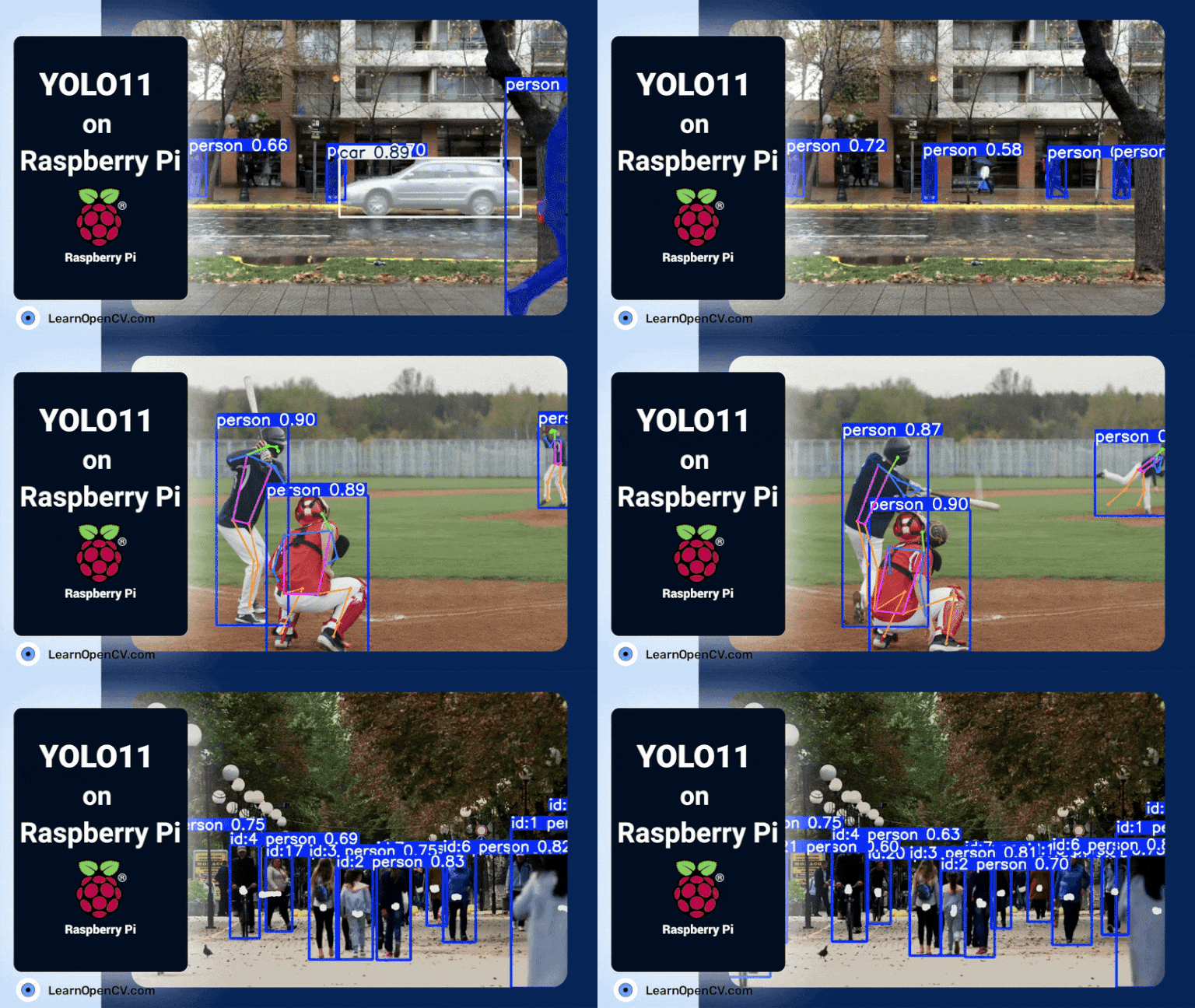
First, we will run the inference using the MNN format, and we will perform object detection and tracking. This is the result:

Now, let’s try to do a segmentation with the OpenVINO format:

Also, we have tried pose estimation with the NCNN format:

We have also tried live detection, tracking, and counting, mimicking a real-time industry project. Here are the results:

As you can see, in your experiments across all the formats, we got an average FPS of about 8 – 10, and there is a very minimal latency that we can’t realize in real time. And we have the perfect combo so far: YOLO11 on Raspberry Pi, which can do any kind of computer vision task with this simple and powerful setup!

Let’s summarize what we have learned so far.

Quick Recap

Edge AI is the Future, and Raspberry Pi is a Powerful, Affordable Enabler: The edge AI market is experiencing explosive growth, demanding solutions that process data locally. The Raspberry Pi, especially the latest Pi 5, emerges as a cost-effective and accessible platform for deploying AI at the edge thanks to its improved processing power and robust community support.

YOLO11 Brings Real-Time Object Detection to Resource-Constrained Devices: YOLO11 stands out as an optimized object detection model specifically designed for edge devices. It achieves remarkable speed and efficiency gains (up to 37% model complexity reduction compared to YOLOv8) while maintaining high accuracy (around 85% mAP), making real-time performance on Raspberry Pi a tangible reality.

Optimization Techniques Unlock Impressive Performance on Raspberry Pi: By employing techniques like NCNN model conversion and hardware-aware quantization, YOLO11 on Raspberry Pi can achieve millisecond-level latency and process video at frame rates of 8-10 FPS or even up to 25+ FPS at lower resolutions. This demonstrates the feasibility of real-time object detection directly on the device.

Edge Deployment Offers Tangible Benefits Beyond Speed: Running YOLO11 on Raspberry Pi brings practical advantages like reduced bandwidth consumption by processing video locally, enhanced data privacy by avoiding cloud data transfers, and near-instant response times crucial for real-time applications in remote or unreliable network environments. This combination democratizes AI, making sophisticated computer vision accessible for various real-world scenarios.

Conclusion

This focus on on-device inference isn’t only about eliminating annoying latency or hefty cloud fees—though those are big perks. More crucially, it’s about democratizing AI. When even a small business or research team on a tight budget can implement robust computer vision, new innovations spring up in every corner of the world. And in an age where edge computing is rapidly becoming the norm, low-cost, high-efficiency object detection solutions like YOLO11 on a Raspberry Pi represent a giant leap toward a future of ubiquitous, intelligent systems.

Ready to get your hands dirty? Don’t forget to check out the more detailed scripts, setup instructions, and supplementary files we’ll provide. Just hit the “Download Code” button to begin your journey into real-time object detection with Raspberry Pi 5 and YOLO11. 

References

Raspberry Pi Documentation

Ultralytics YOLO11 Docs