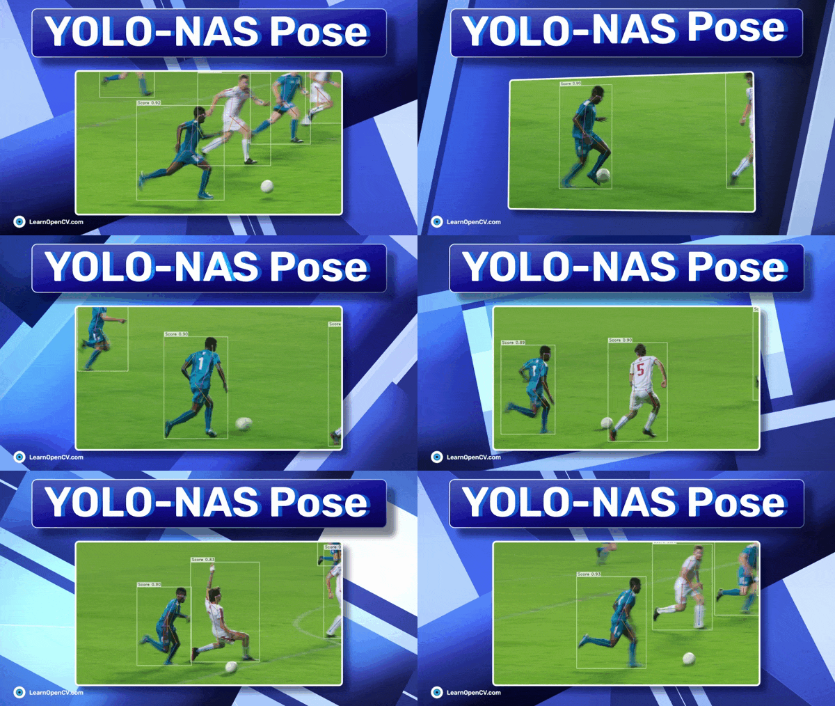
YOLO-NAS Pose models is the latest contribution to the field of Pose Estimation. Earlier this year, Deci garnered widespread recognition for its groundbreaking object detection foundation model, YOLO-NAS. Building upon the success of YOLO-NAS, the company has now unveiled YOLO-NAS Pose as its Pose Estimation counterpart. This Pose model offers an excellent balance between latency and accuracy.
Pose Estimation plays a crucial role in computer vision, encompassing a wide range of important applications. These applications include monitoring patient movements in healthcare, analyzing the performance of athletes in sports, creating seamless human-computer interfaces, and improving robotic systems.
YOLO Master Post – Every Model Explained
Don’t miss out on this comprehensive resource, Mastering All Yolo Models for a richer, more informed perspective on the YOLO series.
YOLO-NAS Pose Model Architecture
The traditional Pose Estimation models follow one of the two approaches:
- Detect all the persons in the scene, then estimate its keypoints and create the pose. A two-stage top-down process.
- Detect all the keypoints in the scene, then generate the pose. A two-stage bottom-up process.
YOLO-NAS Pose does things differently compared to the traditional Pose Estimation models. Instead of first detecting the person and then estimating their pose, it can detect and estimate the person and their pose all at once, in a single step.
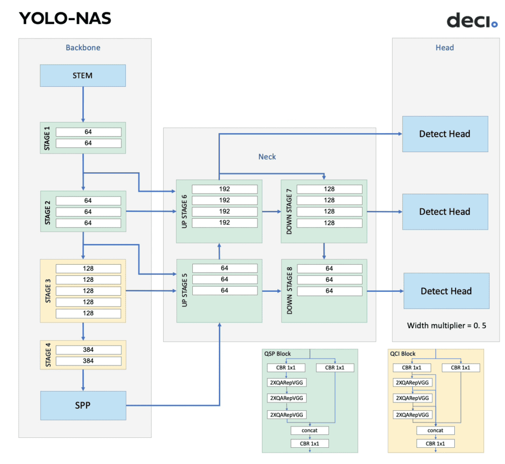
The Pose models are built on top of the YOLO-NAS object detection architecture. Both the Object Detection models and the Pose Estimation models have the same backbone and neck design but differ in the head. The head for YOLO-NAS Pose is designed for its multi-task objective, i.e., detecting a single class object (like a person or an animal) and estimating the pose of the object
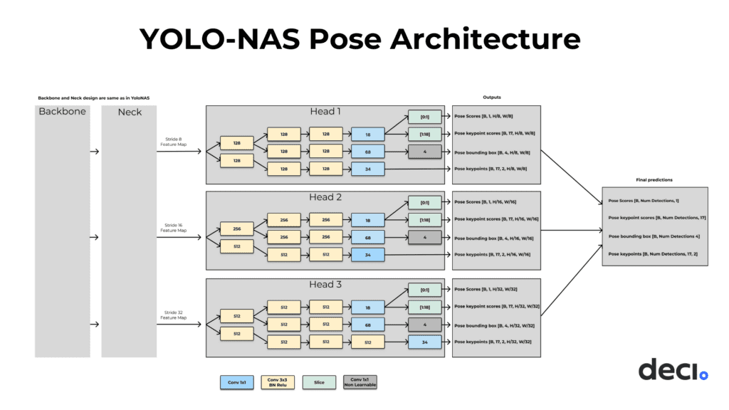
This impressive combination is the result of Deci’s proprietary Neural Architecture Search (NAS) engine, AutoNAC. It navigates the vast architecture search space and returns the best architectural designs. The following are the hyperparameters for the search:
- The number of Conv-BN-Relu blocks for both pose and box regression paths.
- The number of intermediate channels for both paths
- The decision between a shared stem for pose/box regression or distinct stems
The result speaks for itself.
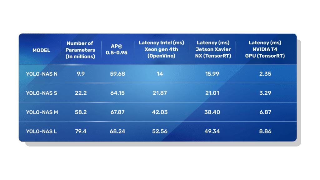
The YOLO-NAS Pose models are evaluated on the COCO Val 2017 Dataset. The model’s accuracy and latency are state-of-the-art. The nano model is the fastest and reaches inference up to 425fps on a T4 GPU. Meanwhile, the large model can reach up to 113 fps.
If we look at edge deployment, the nano and medium models will still run in real-time at 63fps and 48 fps, respectively. But when we look at the medium and large models deployed on Jetson Xavier NX, the speed starts dwindling and reaches 26fps and 20fps, respectively. These are still some of the best results available.
Running Inference On YOLO-NAS Pose
YOLO-NAS Pose models, training pipeline, and notebooks are available in SuperGradients, a PyTorch-based Open Source Vision Library by Deci. You can install SuperGradients via pip.
pip install super-gradients
To run inference, we will import the following Python modules:
torch: importing thePyTorchframework. The foundation on whichSuperGradientsis built.os: Useful for system commands and directory operations.pathlib: Used to get the file paths and path operations.super_gradients: The home of YOLO-NAS Pose models.
import torch
import os
import pathlib
from super_gradients.training import models
from super_gradients.common.object_names import Models
Now we need some images to run inference on. Let’s download these using wget.
urls = [
    "https://mir-s3-cdn-cf.behance.net/project_modules/max_3840/2712bd29493563.55f6ec5e98924.jpg",
    "https://i.pinimg.com/736x/5a/8a/5c/5a8a5c4cd658580ae4719e5c96043541.jpg",
    "https://mir-s3-cdn-cf.behance.net/project_modules/max_1200/4d222729493563.55f6420cd3768.jpg"
]
downloaded_files = []

for index, url in enumerate(urls, start=1):
  os.system(f"wget {url} -O pose-{index}.jpg")
  downloaded_files.append(f"pose-{index}.jpg")
We add a few image URLs in a list, and then loop through the list and download and rename each file using wget, and append the file paths to a new list downloaded_files.
Next, we get the YOLO-NAS Pose models.
model = models.get("yolo_nas_pose_l", pretrained_weights="coco_pose")
device = 'cuda' if torch.cuda.is_available() else 'cpu'
model.to(device)
Using the function get() we download the models. Pass the model name, followed by the path to the weights file. In our case, we are using the NAS Pose Large model with COCO pretrained weights.
And then, load this model to the GPU device, if available. It will tremendously speed up the inference.
Now, use the function predict() to run predictions on the images.
confidence = 0.6
model.predict(downloaded_files[0], conf=confidence).show()
predict() accepts the image and the confidence threshold as input to run inference on the model. Use show() to display the output.
Apart from images, predict() also accepts the following as inputs:
| Path to local image (str) | predict("path/to/image.jpg") |
| Path to images directory (str) | predict("path/to/images/directory") |
| Path to local video (str) | predict("path/to/video.mp4") |
| URL to remote image (str) | predict("https://example.com/image.jpg") |
| 3-dimensional NumPy image ([H, W, C]) | predict(np.zeros((480, 640, 3), dtype=np.uint8)) |
| 4-dimensional NumPy image ([N, H, W, C] or [N, C, H, W]) | predict(np.zeros((480, 640, 3), dtype=np.uint8)) |
| List of 3-dimensional numpy arrays ([H1, W1, C], [H2, W2, C], …) | predict([np.zeros((480, 640, 3), dtype=np.uint8), np.zeros((384, 512, 3), dtype=np.uint8) ]) |
| 3-dimensional Torch Tensor ([H, W, C] or [C, H, W]) | predict(torch.zeros((480, 640, 3), dtype=torch.uint8)) |
| 4-dimensional Torch Tensor ([N, H, W, C] or [N, C, H, W]) | predict(torch.zeros((4, 480, 640, 3), dtype=torch.uint8)) |
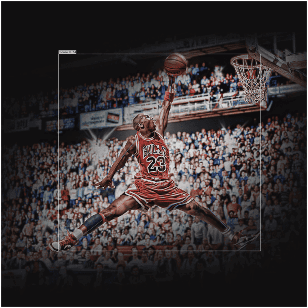
SuperGradients can also save the output instead of displaying it.
output_file = pathlib.Path(downloaded_files[1]).stem + "-detections" + pathlib.Path(downloaded_files[1]).suffix
model.predict(downloaded_files[1], conf=confidence).save(output_file)
Both methods will plot the results on the input image or video. If you just want the results:
preds = model.predict(downloaded_files[2], conf=confidence)
The raw predictions will have the following:
- Bounding Box predictions in XYXY format
- Detection scores for the predicted objects
- 17 Keypoint predictions in XY format
- Confidence scores for each of these keypoints
The initial post-processing step should include applying Non-Maximum Suppression to both the box detections and pose predictions, giving you a collection of high-confidence predictions. Then choose the matching boxes and poses, which together form the model output. Since the model is trained to ensure that box detections and pose predictions occur in the same spatial location, their consistency is maintained.
YOLO-NAS Pose v/s YOLOv8 Pose
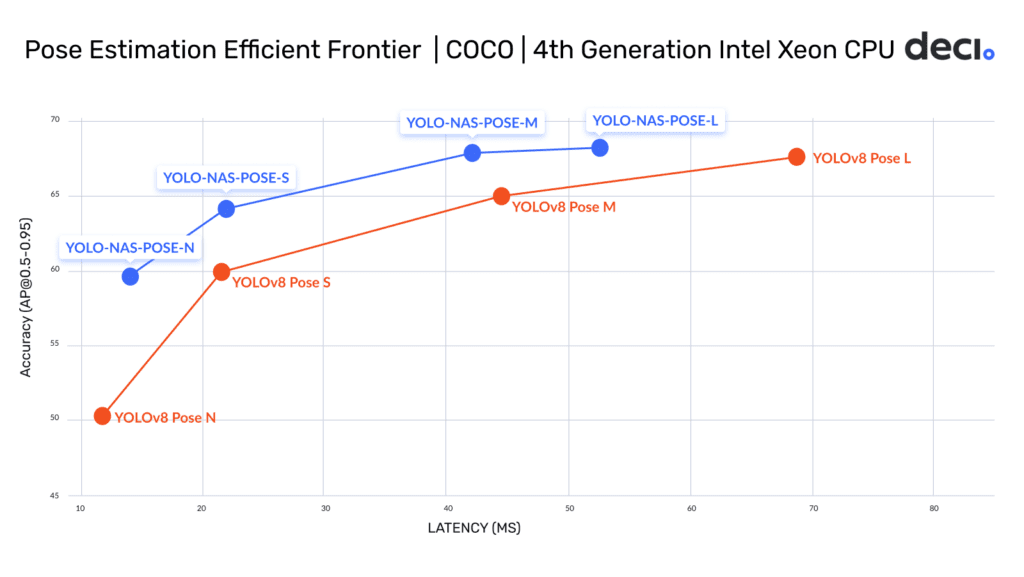
The above graph is the accuracy latency trade-off of the YOLO-NAS Pose and the YOLOv8 Pose models. This space is also known as the efficiency frontier. All the models are evaluated on the COCO Val 2017 Dataset and Intel Xeon 4th gen CPU with 1 batch size and 16-bit floating point operations.
The accuracy of all the YOLO-NAS Pose models is higher than the YOLOv8 Pose models. This can be accredited to AutoNAC’s head designs. Now, let’s talk about specifics:
- The smaller YOLO-NAS Pose models, namely nano and small, although have a higher accuracy, but are slower than the YOLOv8 Pose models.
- The larger YOLO-NAS Pose models, like medium and large, are better in terms of both, accuracy and latency.
Now if we want to dive deeper, here are the results of the YOLO-NAS pose and the YOLOv8 Pose models on the COCO Val 2017 Dataset.
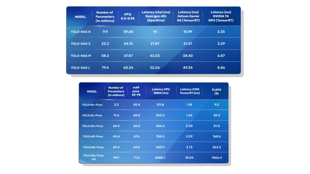
The accuracy of the YOLO-NAS Pose models is always better than their corresponding YOLOv8 Pose model. Let’s take a look at the specifics:
- The number of parameters of the corresponding models are not similar. For example, the NAS Nano has 9.9m parameters, but the v8 Nano has 3.3m parameters. That is a one-third difference.
- Moreover, the inference run hardware is also different. NAS has posted results on a T4 GPU, which was released in September 2018, whereas v8 has posted results on a more recent A100 GPU.
Drop a comment if you’d like me to perform a comparative analysis on both the Pose models.
How Were The Pose Models Trained?
YOLO-NAS Pose Loss Function
To make sure the model learned both tasks effectively, Deci improved the loss functions that were used in training. Instead of just considering the IoU (Intersection over Union) score for assigned boxes, we also incorporated the Object Keypoint Similarity (OKS) score, which compares predicted key points to the actual ones. This change encourages the model to make accurate predictions for both bounding boxes and pose estimation.
Moreover, a direct OKS regression technique was used, which surpasses the traditional L1/L2 loss methods. This approach offers several advantages:
- It operates within a range of 0 to 1, similar to box IoU, indicating how similar the poses are.
- It takes into account the varying levels of difficulty in annotating specific keypoints. Each keypoint is associated with a unique sigma score, which reflects the accuracy of annotation and dataset specifics. The score determines how much the model is penalized for making inaccurate predictions.
- Using a loss function that aligns with the validation metric, which in turn allows for targeting and optimization of the metric.
Training Hyperparameters
Since, YOLO-NAS Pose employs a similar foundational structure as the YOLO-NAS model the pre-trained weights from YOLO-NAS were used to initialize the backbone and neck of our model before proceeding with the final training. Here are the training hyperparameters:
- Training Hardware: Used 8 NVIDIA GeForce RTX 3090 GPUs with PyTorch 2.0.
- Training Schedule: Training was conducted for up to 1000 epochs, with early stopping if there was no improvement in performance over the last 100 epochs.
- Optimizer: Employed AdamW with Cosine LR (Learning Rate) decay, reducing the LR by a factor of 0.05 towards the end of training.
- Weight Decay: A weight decay factor of 0.000001 was applied, excluding bias and BatchNorm layers.
- EMA (Exponential Moving Average) Decay: Used a beta factor of 50 for EMA decay.
- Image Resolution: Images were processed to have a maximum side length of 640 pixels and were padded to a resolution of 640×640 with a padding color of (127, 127, 127).
Augmentations like mosaic data augmentation, random 90-degree rotations, and color augmentations further improved AP by 2.
Conclusion
YOLO-NAS Pose is one of the best Pose Estimation models right now. In this post, we have briefed about the various models, understood the YOLO-NAS Pose model architecture and AutoNAC, and run inference using SuperGradients.

