In this article, we will learn about autoencoders in deep learning. We will show a practical implementation of using a Denoising Autoencoder on the MNIST handwritten digits dataset as an example. In addition, we are sharing an implementation of the idea in Tensorflow.
1. What is An Autoencoder?
An autoencoder is an unsupervised machine-learning algorithm that takes an image as input and reconstructs it using fewer bits. That may sound like image compression, but the biggest difference between an autoencoder and a general purpose image compression algorithm is that in the case of autoencoders, the compression is achieved by learning on a training set of data. While reasonable compression is achieved when an image is similar to the training set used, autoencoders are poor general-purpose image compressors; JPEG compression will do vastly better.
Autoencoders are similar in spirit to dimensionality reduction techniques like principal component analysis. They create a space where the essential parts of the data are preserved while non-essential ( or noisy ) parts are removed.
There are two parts to an autoencoder
- Encoder: This is the part of the network that compresses the input into a fewer number of bits. The space represented by these fewer number of bits is called the “latent-space” and the point of maximum compression is called the bottleneck. These compressed bits that represent the original input are together called an “encoding” of the input.
- Decoder: This is the part of the network that reconstructs the input image using the encoding of the image.
Let’s look at an example to understand the concept better.
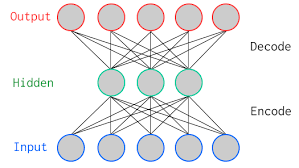
In the above picture, we show a vanilla autoencoder — a 2-layer autoencoder with one hidden layer. The input and output layers have the same number of neurons. We feed five real values into the autoencoder compressed by the encoder into three real values at the bottleneck (middle layer). Using these three real values, the decoder tries reconstructing the five real values we had fed as input to the network.
In practice, there are a far larger number of hidden layers in between the input and the output.
There are various kinds of autoencoders like a sparse autoencoder, variational autoencoder, and denoising autoencoder. In this post, we will learn about a denoising autoencoder.
2. Denoising Autoencoders
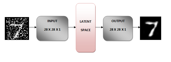
The idea behind a denoising autoencoder is to learn a representation (latent space) that is robust to noise. We add noise to an image and then feed this noisy image as an input to our network. The encoder part of the autoencoder transforms the image into a different space that preserves the handwritten digits but removes the noise. As we will see later, the original image is 28 x 28 x 1 image, and the transformed image is 7 x 7 x 32. You can think of the 7 x 7 x 32 image as a 7 x 7 image with 32 color channels.
The decoder part of the network then reconstructs the original image from this 7 x 7 x 32 image, and voila the noise is gone!
How does this magic happen?
During training, we define a loss (cost function) to minimize the difference between the reconstructed image and the original noise-free image. In other words, we learn a 7 x 7 x 32 space that is noise-free.
3. Implementation of Denoising Autoencoder
This implementation is inspired by this excellent post Building Autoencoders in Keras.
3.1 The Network
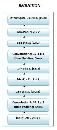
The images are matrices of size 28 x 28. We reshape the image to be of size 28 x 28 x 1, convert the resized image matrix to an array, rescale it between 0 and 1, and feed this as an input to the network. The encoder transforms the 28 x 28 x 1 image to a 7 x 7 x 32 image. You can think of this 7 x 7 x 32 image as a point in a 1568 ( because 7 x 7 x 32 = 1568 ) dimensional space. This 1568 dimensional space is called the bottleneck or the latent space. The architecture is graphically shown below.
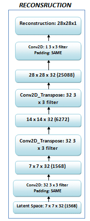
The decoder does the exact opposite of an encoder; it transforms this 1568 dimensional vector back to a 28 x 28 x 1 image. We call this output image a “reconstruction” of the original image. The structure of the decoder is shown below.
Let’s dive into the implementation of an autoencoder using TensorFlow.
3.2 Encoder
The encoder has two convolutional layers and two max pooling layers. Both Convolution layer-1 and Convolution layer-2 have 32-3 x 3 filters. There are two max-pooling layers, each of size 2 x 2.
encoder = Sequential([
    # convolution
    Conv2D(
        filters=32,
        kernel_size=(3,3),
        strides=(1,1),
        padding='SAME',
        use_bias=True,
        activation=lrelu,
        name='conv1'
    ),
    # the input size is 28x28x32
    MaxPooling2D(
        pool_size=(2,2),
        strides=(2,2),
        name='pool1'
    ),
    # the input size is 14x14x32
    Conv2D(
        filters=32,
        kernel_size=(3,3),
        strides=(1,1),
        padding='SAME',
        use_bias=True,
        activation=lrelu,
        name='conv2'
    ),
    # the input size is 14x14x32
    MaxPooling2D(
        pool_size=(2,2),
        strides=(2,2),
        name='encoding'
    )
    # the output size is 7x7x32
])

3.3 Decoder
The decoder has two Conv2d_transpose layers, two Convolution layers, and one Sigmoid activation function. Conv2d_transpose is for upsampling, which is opposite to the role of a convolution layer. The Conv2d_transpose layer upsamples the compressed image twice each time we use it.
decoder = Sequential([
    Conv2D(
        filters=32,
        kernel_size=(3,3),
        strides=(1,1),
        name='conv3',
        padding='SAME',
        use_bias=True,
        activation=lrelu
    ),
    # updampling, the input size is 7x7x32
    Conv2DTranspose(
        filters=32,
        kernel_size=3,
        padding='same',
        strides=2,
        name='upsample1'
    ),
    # upsampling, the input size is 14x14x32
    Conv2DTranspose(
        filters=32,
        kernel_size=3,
        padding='same',
        strides=2,
        name='upsample2'
    ),
    # the input size is 28x28x32
    Conv2D(
        filters=1,
        kernel_size=(3,3),
        strides=(1,1),
        name='logits',
        padding='SAME',
        use_bias=True
    )
])

The resultant encoder-decoder model class is represented as:
# model class definition
class EncoderDecoderModel(Model):
    def __init__(self, is_sigmoid=False):
        super(EncoderDecoderModel, self).__init__()
        # assign encoder sequence
        self._encoder = encoder
        # assign decoder sequence
        self._decoder = decoder
        self._is_sigmoid = is_sigmoid

    # forward pass
    def call(self, x):
        x = self._encoder(x)
        decoded = self._decoder(x)
        if self._is_sigmoid:
            decoded = tf.keras.activations.sigmoid(decoded)
        return decoded
Finally, we calculate the loss of the output using cross-entropy loss function and use Adam optimizer to optimize our loss function.
3.4 Why do we use a leaky ReLU and not a ReLU as an activation function?
We want gradients to flow while we backpropagate through the network. We stack many layers in a system in which there are some neurons whose value drop to zero or become negative. Using a ReLU as an activation function clips the negative values to zero and in the backward pass, the gradients do not flow through those neurons where the values become zero. Because of this the weights do not get updated, and the network stops learning for those values. So using ReLU is not always a good idea. However, we encourage you to change the activation function to ReLU and see the difference.
# define leaky ReLU function
def lrelu(x, alpha=0.1):
    return tf.math.maximum(alpha*x, x)
Therefore, we use a leaky ReLU which instead of clipping the negative values to zero, cuts them to a specific amount based on a hyperparameter alpha. This ensures that the network learns something even when the pixel value is below zero.
3.5 Load the data
Once the architecture has been defined, we load the training and validation data.
As shown below, Tensorflow allows us to easily load the MNIST data. The training and testing data loaded is stored in variables train_imgs and test_imgs respectively. Since it’s an unsupervised task we do not care about the labels.
# load mnist dataset
(train_imgs, train_labels), (test_imgs, test_labels) = tf.keras.datasets.mnist.load_data()

# fit image pixel values from 0 to 1
train_imgs, test_imgs = train_imgs / 255.0, test_imgs / 255.0
3.6 Data Analysis
Before training a neural network, it is always a good idea to do a sanity check on the data.
Let’s see how the data looks like. The data consists of handwritten numbers ranging from 0 to 9, along with their ground truth labels. It has 55,000 train samples and 10,000 test samples. Each sample is a 28×28 grayscale image. Let’s view the data details:
# check data array shapes:
print("Size of train images: {}, Number of train images: {}".format(train_imgs.shape[-2:], train_imgs.shape[0]))
print("Size of test images: {}, Number of test images: {}".format(test_imgs.shape[-2:], test_imgs.shape[0]))
The output is:
Size of train images: (28, 28), Number of train images: 60000
Size of test images: (28, 28), Number of test images: 10000
The visualization of train and test image examples:
# plot image example from training images
plt.imshow(train_imgs[1], cmap='Greys')
plt.show()

# plot image example from test images
plt.imshow(test_imgs[0], cmap='Greys')
plt.show()
plt.close()
Output:
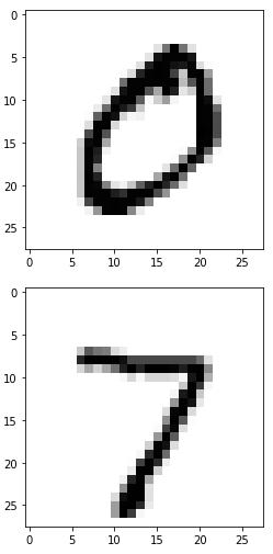
3.7 Preprocessing the data
The images are grayscale and the pixel values range from 0 to 255. We apply the following preprocessing to the data before feeding it to the network.
- Add a new dimension to the train and test images, which will be fed into the network.
# prepare training reference images: add new dimension
train_imgs_data = train_imgs[..., tf.newaxis]

# prepare test reference images: add new dimension
test_imgs_data = test_imgs[..., tf.newaxis]
- Add noise to both train and test images which we then feed into the network. The noise factor is a hyperparamter and can be tuned accordingly.
# add noise to the images for train and test cases
def distort_image(input_imgs, noise_factor=0.5):
    noisy_imgs = input_imgs + noise_factor * np.random.normal(loc=0.0, scale=1.0, size=input_imgs.shape)
    noisy_imgs = np.clip(noisy_imgs, 0., 1.)
    return noisy_imgs

# prepare distorted input data for training
train_noisy_imgs = distort_image(train_imgs_data)

# prepare distorted input data for evaluation
test_noisy_imgs = distort_image(test_imgs_data)
Let’s illustrate the noisy images :
# plot distorted image example from training images
image_id_to_plot = 0
plt.imshow(tf.squeeze(train_noisy_imgs[image_id_to_plot]), cmap='Greys')
plt.title("The number is: {}".format(train_labels[image_id_to_plot]))
plt.show()

# plot distorted image example from test images
plt.imshow(tf.squeeze(test_noisy_imgs[image_id_to_plot]), cmap='Greys')
plt.title("The number is: {}".format(test_labels[image_id_to_plot]))
plt.show()
plt.close()
Output:
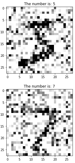
3.8 Train and evaluate the model
The network is ready to get trained. We specify the number of epochs as 25 with batch size of 64. This means that the whole dataset will be fed to the network 25 times. We will be using the test data for validation.
# define custom target function for further minimization
def cost_function(labels=None, logits=None, name=None):
    loss = tf.nn.sigmoid_cross_entropy_with_logits(labels=labels, logits=logits, name=name)
    return tf.reduce_mean(loss)

# init the model
encoder_decoder_model = EncoderDecoderModel()

# training loop params
num_epochs = 25
batch_size_to_set = 64

# training process params
learning_rate = 1e-5
# default number of workers for training process
num_workers = 2

# initialize the training configurations such as optimizer, loss function and accuracy metrics
encoder_decoder_model.compile(optimizer=tf.compat.v1.train.AdamOptimizer(learning_rate=learning_rate),loss=cost_function,metrics=None)

results = encoder_decoder_model.fit(
    train_noisy_imgs,
    train_imgs_data,
    epochs=num_epochs,
    batch_size=batch_size_to_set,
    validation_data=(test_noisy_imgs, test_imgs_data),
    workers=num_workers,
    shuffle=True
)
After 25 epochs, we can see our training loss and validation loss is quite low, which means our network did a pretty good job. Let’s now see the loss plot between training and validation data using the introduced utility function plot_losses(results).
3.10 Training Vs. Validation Loss Plot
We’ve defined the utility function for plotting the losses:
# funstion for train and val losses visualizations
def plot_losses(results):
    plt.plot(results.history['loss'], 'bo', label='Training loss')
    plt.plot(results.history['val_loss'], 'r', label='Validation loss')
    plt.title('Training and validation loss',fontsize=14)
    plt.xlabel('Epochs ',fontsize=14)
    plt.ylabel('Loss',fontsize=14)
    plt.legend()
    plt.show()
    plt.close()

# visualize train and val losses
plot_losses(results)
The result is:
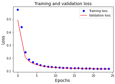
From the above loss plot, we can observe that the validation loss and training loss steadily decrease in the first ten epochs. This training loss and the validation loss are also very close to each other. This means that our model has generalized well to unseen test data.
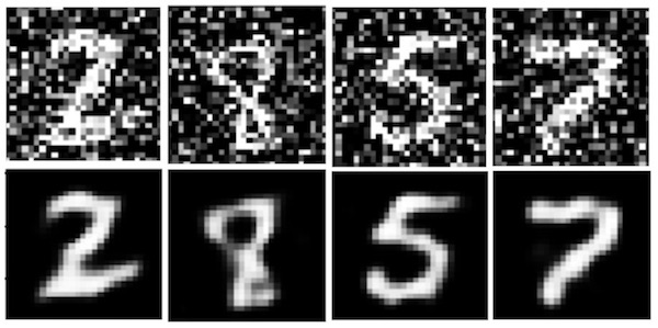
We can further validate our results by observing the original, noisy and reconstruction of test images.
3.11 Results
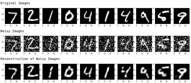
From the above figures, we can observe that our model did a good job in denoising the noisy images that we had fed into our model.






100K+ Learners
Join Free OpenCV Bootcamp3 Hours of Learning