Stereo Vision and Depth Estimation using OpenCV AI Kit

Gone are the days when setting up the proper hardware and software for a stereo vision project was arduous. Thanks to OpenCV and Luxonis, you no longer have to worry about cumbersome initial setups.

This is the second article of the OAK series. Previously we have covered the installation of DepthAI API and introduced a basic pipeline. This post will explain why we need two cameras to estimate depth. Then we will build a pipeline to calculate depth using OAK-D or OAK-D Lite. Following are some key terminologies that you will come across in this article.

Check out more articles from the OAK series.

• Stereo Vision and Depth Estimation using OpenCV AI Kit
• Object detection with depth measurement using pre-trained models with OAK-D

1. The geometry of stereo vision
2. Hurdles in depth estimation
3. Depth estimation pipeline
4. Code explanation
5. Demonstration
6. Limitations

The Geometry of Stereo Vision

Stereo vision is one of the ways humans perceive depth. The word stereo means “two.” We look at the same scene from two viewpoints to get a sense of depth. Humans perceive depth through several other means, but that is a discussion for another day. 

The human vision system inspired computer stereo vision systems. With OAK-D, even the camera distance is close to the distance between human eyes! 

Let’s recap the theory of image formation before we dive into stereo vision.

The Coordinate Systems

An image is a 2D projection of a 3D object from the real world to an image plane. We use the following coordinate systems to describe an imaging setup.

1. World coordinate (3D, unit: meters)
2. Camera coordinate (3D, unit: meters)
3. Image plane coordinate (2D, unit: pixels)

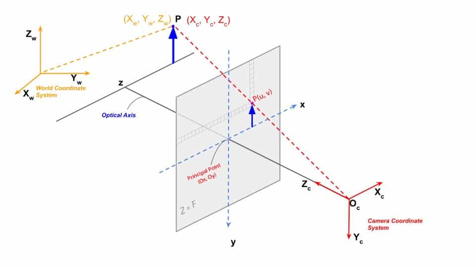
Fig 1: Coordinate systems in an imaging system

Mapping world coordinates to pixel coordinates tells us how far the object is from the camera perspective. To map or relate these coordinates, we need to know the camera’s parameters (e.g., the focal length).

What is Camera Calibration?

The process of obtaining the lens and image sensor parameters is called Camera Calibration. There are two kinds of parameters – internal and external. We have a detailed post on camera calibration.

We can evaluate the Transformation Matrix with these parameters. It maps real-world coordinates to pixel coordinates. Our earlier article on the geometry of image formations has more details.

How is Depth Calculated?

Let us consider that a camera captures the image of a real-world point Po, where P_o(x, y, z) is the position of the point in the real world and P(u, v) in the image plane.

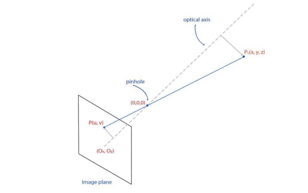
Fig 2: Pinhole camera – image formation

The perspective projection equations can be written as follows for a calibrated system. 

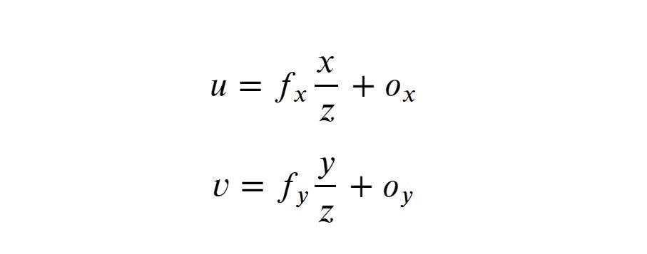
Where, 

• f_x, f_y, u, v, O_x, O_y are known parameters in pixel units. 
• The pixels in the image sensor may not be square, so we may have two different focal lengths f_x and f_y. 
• (O_x, O_y) is the point where the optical axis intersects the image plane.

Since we have only two equations, we cannot find the three unknown variables, x, y, and z. To find them, we need two cameras. Another identical camera is positioned in a stereo system, as shown below. Both cameras are assumed to have no lens distortion

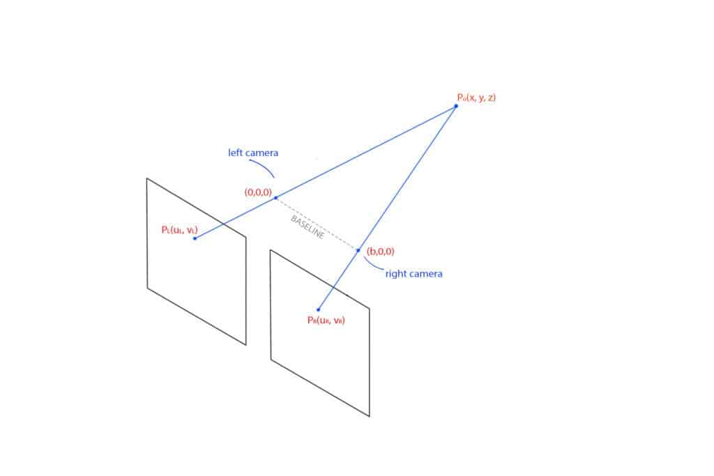
Fig 3: Image formation in a stereo setup

• The line between the centers of the cameras is called the baseline. 
• P_L(u_L, v_L) and P_R(u_R, v_R) are projections of point P_o in the left and right image plane respectively.

This setup gives us the following four equations.

Solving these equations, we obtain x, y, and z as follows.

Here, the z is the depth of the point from the camera. It is directly proportional to the baseline.

What is Disparity?

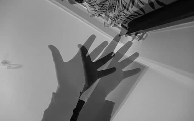
If you look closely at the two images captured by the mono cameras, you will observe that the images are not identical. The disparity is easily observed by combining the two images into a single image with 50% contribution from each image. There is a difference in the positions of corresponding points. This difference is called Disparity.

The disparity is inversely proportional to depth.

Finding the corresponding points in the second image can be achieved using template matching or similar methods. An image captured by high-resolution cameras has millions of pixels. Hence, it will be highly process-intensive if we do it for the entire picture. Luckily, our cameras are calibrated, and images are rectified. Therefore, we only need to search along the horizontal line where P_L lies.

Hurdles in Depth Estimation

Depth estimation in practice is not as smooth as a peeled egg. As discussed above, we derived the equation for depth with the following assumptions. 

1. Cameras are leveled.
2. Images are coplanar.
3. No optical distortion.

However, it is tough to attain ideal situations in a stereo pair. The cameras are rarely aligned, and the images are not coplanar. This is fixed by stereo rectification. 

Stereo rectification is the reprojection of the left and right image planes onto a common plane parallel to the baseline. We will discuss how to carry out the operation in the pipeline below. Optical distortion is fixed with the help of camera parameters obtained from calibration.

Depth Estimation Pipeline

Previously, we showed how to create a pipeline to access the mono cameras of an OAK-D device. We will improve upon it by adding a stereo depth node to the pipeline, as shown below.

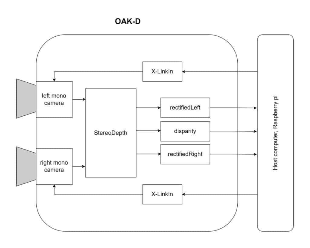
Fig 4: Depth estimation pipeline

A stereo-depth node has the following outputs.

• Rectified left
• Synced left
• Depth
• Disparity
• Rectified right
• Synced right

But in our case, we are concerned about rectifiedLeft, disparity, and rectifiedRight. These outputs are enough to generate the disparity map and display left-right views. So without further ado, let’s get started with the code.

Click here to download the source code to this post

Import Libraries

import cv2
import depthai as dai
import numpy as np

We have already discussed the first two functions in the introductory blog post. If you face difficulty understanding, please do read our Introduction to OAK-D and DepthAI

Function to extract frame

It queries the frame from the queue, transfers it to the host, and converts it to a NumPy array.

def getFrame(queue):
    # Get frame from queue
    frame = queue.get()
    # Convert frame to OpenCV format and return
    return frame.getCvFrame()

Function to select mono camera

We create a node to the pipeline, set the resolution, and then set the board socket to the mono camera.

def getMonoCamera(pipeline, isLeft):
    # Configure mono camera
    mono = pipeline.createMonoCamera()

    # Set Camera Resolution
    mono.setResolution(dai.MonoCameraProperties.SensorResolution.THE_400_P)
    if isLeft:
        # Get left camera
        mono.setBoardSocket(dai.CameraBoardSocket.LEFT)
    else:
        # Get right camera
        mono.setBoardSocket(dai.CameraBoardSocket.RIGHT)
    return mono

Function to configure stereo pair

This function generates a stereo node. It takes left and right camera streams as inputs and generates the outputs discussed above. After creating the node, we set the left-right check to True for better occlusion handling. This flag tells the system to compute and combine disparities in L-R and R-L directions, discarding invalid disparity values. You can play with this flag and notice the noisy output when you set the flag to False. Finally, we provide the camera outputs as input to the stereo node.

def getStereoPair(pipeline, monoLeft, monoRight):

    # Configure stereo pair for depth estimation
    stereo = pipeline.createStereoDepth()

    # Checks occluded pixels and marks them as invalid
    stereo.setLeftRightCheck(True)

    # Configure left and right cameras to work as a stereo pair
    monoLeft.out.link(stereo.left)
    monoRight.out.link(stereo.right)

    return stereo

Mouse callback function

Just a mouse callback function defined to record the pixel coordinate of a point when we click on it. 

def mouseCallback(event, x, y, flags, param):
    global mouseX, mouseY
    if event == cv2.EVENT_LBUTTONDOWN:
        mouseX = x
        mouseY = y

Main function

The variables mouseX and mouseY are declared to hold pixel coordinates of a clicked point. We are going to use it to demonstrate the correspondence scan line. The initialization part is pretty much self-explanatory. We are instantiating the pipeline object, setting up left and right cameras, and calling the getStereoPair() function to set up the stereo pair. 

if __name__ == '__main__':
    mouseX = 0
    mouseY = 640

    # Start defining a pipeline
    pipeline = dai.Pipeline()

    # Set up left and right cameras
    monoLeft = getMonoCamera(pipeline, isLeft=True)
    monoRight = getMonoCamera(pipeline, isLeft=False)

    # Combine left and right cameras to form a stereo pair
    stereo = getStereoPair(pipeline, monoLeft, monoRight)

Link stereo outputs to X-LinkOut node

As we have discussed above, we will focus on three outputs of stereo node, disparity, rectifiedLeft, and rectifiedRight. We need to connect these outputs to the X-LinkOut node because X-Link is the node or mechanism through which the device communicates. The code flow is,

• Create respective x-LinkOut nodes
• Assign respective stream names
• Link stereo outputs to the x-LinkOut nodes as inputs

    xoutDisp = pipeline.createXLinkOut()
    xoutDisp.setStreamName("disparity")

    xoutRectifiedLeft = pipeline.createXLinkOut()
    xoutRectifiedLeft.setStreamName("rectifiedLeft")

    xoutRectifiedRight = pipeline.createXLinkOut()
    xoutRectifiedRight.setStreamName("rectifiedRight")

    stereo.disparity.link(xoutDisp.input)
    stereo.rectifiedLeft.link(xoutRectifiedLeft.input)
    stereo.rectifiedRight.link(xoutRectifiedRight.input)

Transfer pipeline to OAK-D

Once we have all the nodes linked properly, we can transfer the pipeline to the device (OAK-D). We start by acquiring the output queue of the streams we named earlier. 

• Each queue is set to hold a maximum of 1 frame/message at a time.
• The argument blocking = False means overwrite the last frame once the queue is full. We don’t want to store the last frame as it is not required.

The disparityMultiplier is defined to map the disparity values in the range 0 – 255. This is done for color mapping the output as the OpenCV function expects the values in this range.

   with dai.Device(pipeline) as device:
        # Output queues will be used to get the rgb frames and nn data 
        from the outputs defined above
        disparityQueue = device.getOutputQueue(name="disparity", 
                                              maxSize=1, blocking=False)
        rectifiedLeftQueue = device.getOutputQueue(name="rectifiedLeft", 
                                              maxSize=1, blocking=False)
        rectifiedRightQueue=device.getOutputQueue(name="rectifiedRight", 
                                              maxSize=1, blocking=False)

        # Calculate a multiplier for color mapping disparity map
        disparityMultiplier = 255 / stereo.getMaxDisparity()

        cv2.namedWindow("Stereo Pair")
        cv2.setMouseCallback("Stereo Pair", mouseCallback)

        # Variable use to toggle between side by side view and one frame 
        view.
        sideBySide = False

Mainloop

We acquire the disparity frame from the queue using the pre-defined function getFrame. The frame is then multiplied by the disparityMultiplier to map the values in the range 0 – 255. We use the JET colormap to visualize the output. This colormap has colors ranging from cool (blue) to hot (red.).

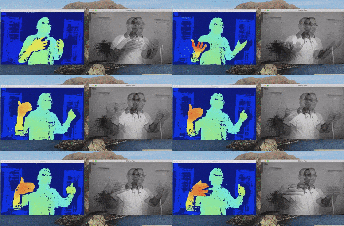
The rest of the code is pretty much self-explanatory. We acquire the left and right frames from their respective queues. It undergoes horizontal stacking or overlapping depending upon the toggle status. Finally, we have two windows as outputs: the disparity map and the mono camera streams.

        while True:
            # Get the disparity map.
            disparity = getFrame(disparityQueue)

            # Colormap disparity for display.
            disparity = (disparity * 
                         disparityMultiplier).astype(np.uint8)
            disparity = cv2.applyColorMap(disparity, cv2.COLORMAP_JET)

            # Get the left and right rectified frame.
            leftFrame = getFrame(rectifiedLeftQueue);
            rightFrame = getFrame(rectifiedRightQueue)

            if sideBySide:
                # Show side by side view.
                imOut = np.hstack((leftFrame, rightFrame))
            else:
                # Show overlapping frames.
                imOut = np.uint8(leftFrame / 2 + rightFrame / 2)
            # Convert to RGB.
            imOut = cv2.cvtColor(imOut, cv2.COLOR_GRAY2RGB)
            # Draw scan line.
            imOut = cv2.line(imOut, (mouseX, mouseY), 
                            (1280, mouseY), (0, 0, 255), 2)
            # Draw clicked point.
            imOut = cv2.circle(imOut, (mouseX, mouseY), 2, 
                            (255, 255, 128), 2)
            cv2.imshow("Stereo Pair", imOut)
            cv2.imshow("Disparity", disparity)

            # Check for keyboard input
            key = cv2.waitKey(1)
            if key == ord('q'):
                # Quit when q is pressed
                break
            elif key == ord('t'):
                # Toggle display when t is pressed
                sideBySide = not sideBySide

Demonstration

Limitations

Depth estimation in OAK-D (or any other stereo vision setup) suffers from the following issues.

1. The scene must have texture, and it should not be repetitive.

For surfaces having no texture, finding the corresponding point becomes difficult. The same situation occurs when the texture has repetitive patterns.

2. Works in a specific distance range.

The objects cannot be too far from the camera. As we have discussed earlier, the disparity is inversely proportional to depth. The disparity reduces when the object moves further away from the cameras and the images look identical. The theoretical maximum depth OAK-D can look at is 38.4 meters. In practice, we should trust it up to about 20 meters. 

Moreover, it fails when the object is too close as well. The disparity is large if the object is very close to the camera. The width of the camera frame is 1280 pixels, but it is computationally expensive to search over 1280 pixels for corresponding points. The DepthAI API searches for corresponding points over a small disparity range of 96 pixels, corresponding to 69 centimeters. This significantly speeds up depth estimation time, but it also means that objects too close to the camera will not have the correct depth estimate. 

You can enable the Extended Disparity mode in OAK-D to reduce the minimum depth to 35 centimeters. In this mode, the API searches over a disparity of 191 pixels. The frame rate will drop when you enable Extended Disparity. There ain’t no such thing as a free lunch.

Conclusion

So that’s all about depth estimation using an OAK-D or OAK-D Lite. I hope you enjoyed the post and learned something new. Check out our OpenCV community’s exciting projects and build your own! 

The next post in this series will cover the pipeline for object detection.

References

• Get an OAK-D
• Get an OAK-D Lite
• DepthAI Docs
• Image formation
• Camera calibration
• Color Map